


Acoustic radiation from the submerged circular cylindrical shell treated with active constrained layer damping
[Yuan Li-Yuna), b) , Xiang Yu†a), b)  , Lu Jing
a), b) , Jiang Hong-Huaa) ]
, Lu Jing|
|


†Corresponding author. E-mail: xiang_yu@126.com
*Project supported by the National Natural Science Foundation of China (Grant Nos. 11162001, 11502056, and 51105083), the Natural Science Foundation of Guangxi Zhuang Autonomous Region, China (Grant No. 2012GXNSFAA053207), the Doctor Foundation of Guangxi University of Science and Technology, China (Grant No. 12Z09), and the Development Project of the Key Laboratory of Guangxi Zhuang Autonomous Region, China (Grant No. 1404544).
Based on the transfer matrix method of exploring the circular cylindrical shell treated with active constrained layer damping (i.e., ACLD), combined with the analytical solution of the Helmholtz equation for a point source, a multi-point multipole virtual source simulation method is for the first time proposed for solving the acoustic radiation problem of a submerged ACLD shell. This approach, wherein some virtual point sources are assumed to be evenly distributed on the axial line of the cylindrical shell, and the sound pressure could be written in the form of the sum of the wave functions series with the undetermined coefficients, is demonstrated to be accurate to achieve the radiation acoustic pressure of the pulsating and oscillating spheres respectively. Meanwhile, this approach is proved to be accurate to obtain the radiation acoustic pressure for a stiffened cylindrical shell. Then, the chosen number of the virtual distributed point sources and truncated number of the wave functions series are discussed to achieve the approximate radiation acoustic pressure of an ACLD cylindrical shell. Applying this method, different radiation acoustic pressures of a submerged ACLD cylindrical shell with different boundary conditions, different thickness values of viscoelastic and piezoelectric layer, different feedback gains for the piezoelectric layer and coverage of ACLD are discussed in detail. Results show that a thicker thickness and larger velocity gain for the piezoelectric layer and larger coverage of the ACLD layer can obtain a better damping effect for the whole structure in general. Whereas, laying a thicker viscoelastic layer is not always a better treatment to achieve a better acoustic characteristic.
The structural-acoustic coupled vibration problem of submerged cylindrical shells, which are widely used in submarines, torpedoes, and other underwater vehicles, has received a great deal of attention. A major current focus on those studies is how to ensure a quite low level of acoustic radiation from those structures. Up till now, many researchers have attempted to layer the viscoelastic or piezoelectric material sublayer on the internal surface of the underwater structures to resist the vibration and noise. Hasheminejad and Rajabi[1] found that the acoustic scattering caused by a plane incident wave could be cancelled when a piezoelectric layer was adhered to the internal surface of an orthotropic cylindrical shell. However, quite a high level of the energy input was usually required to obtain a better damping effect due to the tiny piezoelectric coefficients. Moreover, the reliability of this kind of treatment was rather poor due to the control spillover or breakdown voltage of the piezoelectric layer. Ruzzene et al.[2, 3] treated passive constrained layer damping (i.e., PCLD) on the longitudinal ribs of a cylindrical shell to restrain the acoustic radiation, and better damping effects were achieved. Meanwhile, Saravanan et al.[4] found the damping factors of the whole structures were proved to be enhanced when the PCLD treatment was applied. Unfortunately, the flexibility of the PCLD treatment was insufficient since they could not be self-adaptive to the working condition. Recently, some researchers[5, 6] declared that the active constrained layer damping (i.e. ACLD), which replaced the constrained layer of the PCLD structure with the piezoelectric material, could achieve a better damping effect than the traditional active control (i.e., treating the piezoelectric material on the structure) or PCLD treatment due to its low energy input and being highly self-adaptive. Ro and Baz[5] located some ACLD blocks on an elastic plate to attenuate the noise of a rectangular acoustic cavity with five rigid walls, and good damping effect was acquired. Subsequently, Ray and Balaji[6] employed some ACLD blocks on a cylindrical panel, in order to reject the noise of the same acoustic cavity as mentioned in Ref. [5]. However, there remains a need for further work on the acoustic problem of submerged structures with ACLD treatment, since little work was done on the acoustic characteristic of them.
By convention, the methods adopted to deal with the acoustic-structural problems are numerical methods such as the finite element method (FEM), boundary element method (BEM) or finite/boundary element method. Soize[7] pointed out that although FEM and BEM were proved to be mature and convenient enough to operate, they still tended to be inaccurate when handling issues in the medium high frequency range. Moreover, as expected by Amini andWilton, [8] applying those methods, the solving process would turn out to be much more difficult and complex, since the corresponding transformation should be done into the conventional Helmholtz boundary integral equation to guarantee the solution uniqueness of the Helmholtz external problem. From this point of view, those numerical methods were not always precise and convenient enough to demonstrate the common acoustic characteristic of structures in the whole frequency band. Hence, analytical representations of the acoustic pressure for some simple underwater structures are always pursued by many scholars. To date, analytical representations of the acoustic pressure of single layer cylindrical shells with ribs or deck-type internal plates have been achieved.[9– 14] Among them, a finite length cylindrical shell model was mainly developed to obtain the sound pressure of an underwater cylindrical shell by introducing two infinite rigid baffles at the ends of the shell. However, as the infinite rigid baffles would change the real shape of the external liquid field, a little deviation might be brought in that model. Thus, hemi-spherical or flat plate rigid baffles gradually replaced the conventional infinite ones to obtain a more accurate solution.[13– 15] As for the solution for the acoustic pressure of submerged laminated cylindrical shells, numerical methods such as FEM, BEM, and FEM/BEM are still the major choices. Recently in the last twenty years, a virtual source simulation technique, which was based on the superposition principle and the uniqueness theorem for the Helmholtz problem, has been proposed and proved to be effective for solving the acoustic boundary value problem. This technique to solve the acoustic radiation and scattering problems for structures was developed, and good approximate precision was achieved.[16– 19] Up to now, the virtual source simulation technique has been developed to be a mature method of computing the acoustic boundary value problem. According to the number of the acting positions and the density function for the virtual sources, this technique could be mainly classified into four types: a one-point multipole method, a multi-point monopole method, a multi-point dipole method, and a multi-point multipole method. As for the one-point multipole method, the density function was usually expressed in the form of some spherical wave functions. Hence, the convergent velocity for this method is dependent on the geometric shape of the surface of the vibrating body. When the geometric shape of the vibrating boundary seriously deviates from a sphere, the convergent velocity of the one-point multipole method tends to be slow. In that case, the other three methods are preferred to be adopted.[17, 18] Meanwhile, to avoid the singularity of the acoustic radiation, the virtual points are assumed to be located in the inside or in the outside of the real structure, and on a virtual boundary in a similar shape with the real boundary to guarantee the precision and efficiency.[19]
As mentioned above, ACLD is generally considered to be a better damping treatment on vibration and acoustic suppression. Thus, up to now, considerable investigations, including modeling, control strategy and analysis method etc., have been placed on ACLD cylindrical shells. Focusing on the geometric characteristic of an ACLD cylindrical shell, Saravanan et al.[4] developed a semi-analytical finite element model and used the FEM to demonstrate its dynamic characteristic. Lee and Kim[20] proposed a spectral finite element for ACLD beams. The corresponding spectral finite element method (SFEM) mentioned in the paper was more efficient than conventional FEM. However, it turned out to be difficult to establish the spectral finite element for complex structures such as plates and shells. Shen[21] developed the dynamic differential ordinary equations for the PCLD or ACLD shell. Baz and Chen[22] derived the axis-symmetric control equations of an ACLD cylindrical shell and explored the boundary control strategy for the shell. To date, by virtue of the precise integral method with high accuracy, a transfer matrix method has been explored for solving the dynamic problem of ACLD cylindrical shells.[23– 25] According to this method, when the external excitation can be expressed in the form of the Fourier series expansion in the circumferential direction, the radial displacement and its derivation of the point at the surface of the cylindrical shell can be resolved, which makes it possible and convenient to settle the acoustic radiation pressure for submerged ACLD cylindrical shells.
In this paper, the transfer matrix method is further developed for the acoustic radiation from a submerged cylindrical shell with ACLD. Firstly, the control equations of the shell are expressed in the frequency domain. Then, an analytical solution is given for the radiation acoustic pressure by a multi-point multipoles method with undetermined coefficients. Next, applying the coupling condition, these coefficients are determined. After that, a sound pressure level at an arbitrary point in the external liquid field can be provided. Finally, damping effects of different parameters of the ACLD treatment on the acoustic radiation of the sandwich cylindrical shell are discussed.
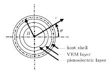
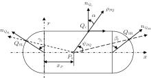
As shown in Figs. 1 and 2, a cylindrical shell fully treated with ACLD is immerged in the liquid. The radius, thickness and length of the host shell are expressed by R1, h1, L respectively. The thickness and radius for the viscoelastic layer are h2 and R2. As for the piezoelectric layer they are denoted by h3 and R3. In this paper, only the inverse piezoelectric effect is considered for the piezoelectric layer, which is transversely isotropic and polarized in the radial direction. Meanwhile, the piezoelectric layer is assumed to be thin enough. Hence, the radial component of the electric field intensity Ez could be taken to be a constant. The electric field intensities and the piezoelectric effect in the other two directions could be neglected also.
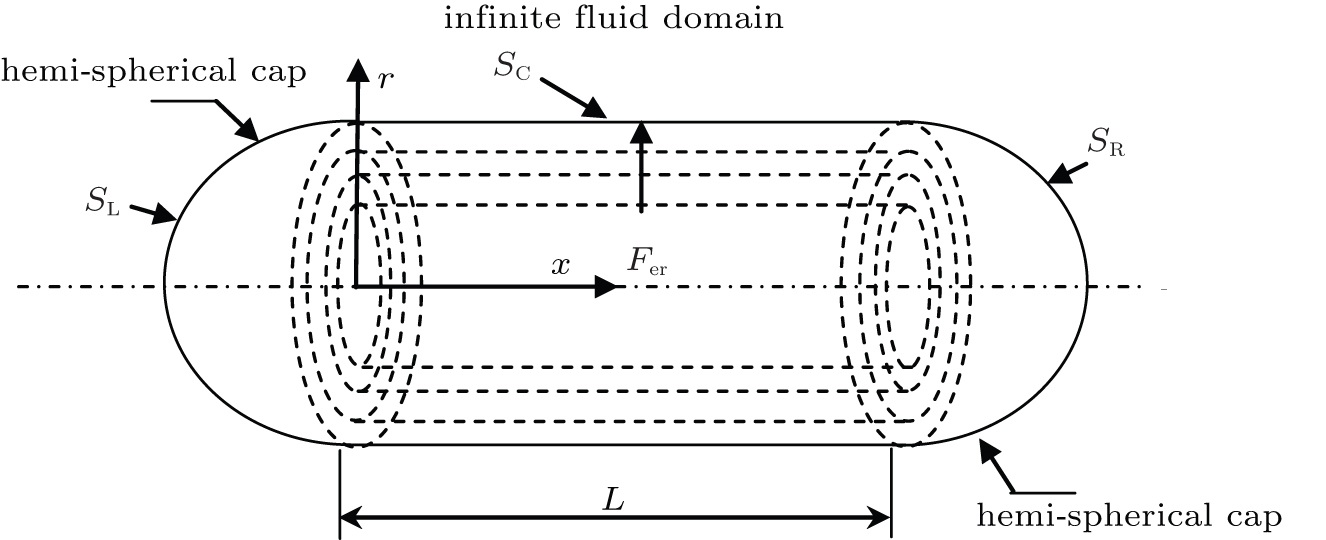 | Fig. 1. Submerged ACLD cylindrical shell with hemi-spherical end caps. |
 | Fig. 2. Cross section for the ACLD cylindrical shell. |
Like Refs. [13] and [14], two semi-spherical rigid baffles are linked at the ends of the cylindrical shell in Fig. 1. Meanwhile, a uniform feedback control voltage is applied to the piezoelectric layer, which means that the distribution function of the control voltage in the circumferential direction, i.e., R(θ ), is equal to unit one. In this case, the electric field intensity in the piezoelectric layer is[21]

in which, kp and kd denote the feedback gain coefficients of the radial displacement and velocity respectively, w(x0, θ 0) is the amplitude of the radial displacement at the feedback referring point with the coordinate (x0, θ 0), eiω t the time factor, and ω the angular frequency for the external harmonic excitation.
According to the thoughts and operations described in Ref. [25], by expanding the physical variables in the control equations of the host shell and the piezoelectric layer in the form of Fourier series expansion in the circumferential direction, and replacing the components of those variables by the dimensionless ones, after derivation and arrangement, the first order ordinary differential matrix control equation for the two layers can be derived respectively. Then, based on the method developed in Ref. [23], by considering the interaction between the viscoelstic layer and the host shell or the piezoelectric layer, by reducing some intermediate variables and through processing, the control equation of the ACLD cylindrical shell in the frequency domain can be yielded as follows:[25]

where ξ = x/L,
represents the integrated state vector of the ACLD cylindrical shell without considering the piezoelectric effect;

is the dimensionless vector of the external harmonic excitation vector; FV denotes the generalized active control force vector acting on the piezoelectric layer, which has been given in Ref. [25]; Ā , B̄ are called the coefficient matrices, and their components, together with 


It is worth pointing out that the dynamic problem of an arbitrary ACLD cylindrical shell can be described by a set of matrix equations in the form of Eq. (2) corresponding to the different values of circumferential wave number n (n = 0, 1, … , ∞ ). Meanwhile, the state variable in each of Z, F, and FV is the dimensionless n-th component of the Fourier series expansion in the circumferential direction for the real physical variable.
In addition, the inhomogeneous terms appearing on the right-hand side of Eq. (2) consist of vectors F and FV · w(x0, θ 0). As for the shell shown in Fig. 1, F is composed of two parts: one is the determined mechanical external excitation vector Fer, and the other is the undetermined acoustic pressure vector P (P = L {0, 0, 0, 0, 0, 0, p, 0, 0, 0, 0, 0}T/K(1), p is the acoustic pressure). Because P together with the term w(x0, θ 0) is dependent on the solution of Eq. (2), the solution of Eq. (2) is difficult to obtain. When F merely comprises Fer, w(x0, θ 0) can be obtained by an extended homogeneous capacity precision integration method and superposition principles, and then Eq. (2) could be resolved successfully.[25] Based on Ref. [25], suppose that the acoustic pressure could be expressed in an analytical form as a sum of the Fourier series with wave numbers in the circumferential direction, the acoustic radiation problem for cylindrical shells shown in Fig. 1 should be solved as well.
Under the harmonic excitation, the acoustic pressure p(r) at any point Q(r) in the liquid field shown in Fig. 1 satisfies the following Helmholtz equation:

where, k = ω /c0 is the wave number, c0 is the sound propagation velocity in the liquid medium.
To ensure the solution uniqueness for Eq. (3), p(r) should meet the Summerfield radiation condition in the far liquid field as well, that is,

Meanwhile, on the liquid-solid interaction surface, Neumann boundary condition is also given as

where rs is the position vector of the point on the interaction surface S, vr (rs) is its normal velocity, while ρ 0 represents the density of the liquid medium.
When the acoustic source is a point sound source located at P, the solution of Eq. (3), which meets Eq. (4), could be yielded in the spherical coordinate system as[26]
in which ρ PQ is the radius vector from the spherical center point Q to the source point P; ψ PQ and ϕ are the polar angle and circumferential angle in the spherical coordinate system respectively; 


Unfortunately, the concrete acoustic source is not always composed of some real point sources. According to the internal source density simulation technique[16– 19, 27] for the acoustic problem of the revolution cavity and by employing superposition principles, a multi-point multipole method is adopted to deal with the radiation acoustic pressure. Generally speaking, these virtual point sources should be assumed to be located in the inside or outside of the real structure to avoid singularity. Hence, in the present paper, the virtual point source is assumed to be located on the axial line of the cylindrical shell. Meanwhile, this kind of location strategy could be a convenient one for programming. In that case, the acoustic pressure caused by each virtual sound source could be expressed in the form of the sum of some wave function series as shown in Eq. (6). Then, by adjusting the density of these wave functions, i.e., the coefficient Bln for each virtual sound source, the real acoustic source could be simulated and the approximate results of the acoustic pressure could be obtained. The detailed steps are given as follows.
Applying a convenient way, supposing that some virtual point sources marked as Pk (xk, 0) are located eventually along the axial line of the cylindrical shell shown in Fig. 3, referring to Eq. (6) and combining with superposition principles, the acoustic pressure at a field point Q could be written as
where NP denotes the total number of the virtual point sources, 

and 
 | Fig. 3. Schematic diagram of the meridian plane at the fluid-solid interface. |
According to Eqs. (7) and (8), the acoustic pressure of Q is represented by the unknown coefficients
where SL, SR, SC represent the interaction surfaces between the liquid field and the left semi-spherical rigid baffle, the right one, and the cylindrical shell respectively. Meanwhile, for the shell of revolution, normal partial derivative of one of the components of acoustic pressure could be deduced as

where, α is the angle between the normal vector npkQ and the vector ρ PkQ. Equation (10) can be further developed for the shell shown in Fig. 3. For the limitation of space, the detailed formulations about it at any point on SL, SR, or SC are derived in Appendix A, which are expressed by Eq. (A1), Eq. (A2), and Eq. (A3) respectively.
It can be seen from Eq. (9) that
Applying the extended homogeneous capacity precision integration method, for a given inhomogeneous term appearing in Eq. (2), the radial displacement caused by it can be solved. Taking the generalized active force FV (known) for example, the detailed process of solving Eq. (2) is described in the following.
Firstly, FV is approximated by a quadratic polynomial vector function

Then, by extended homogeneous capacity processing, equation (2) could be written as

As demonstrated in Ref. [23], equation (12) can be solved by applying precision integration. Hence the radial displacement at any point of the base shell can be obtained.
Assume the radial displacement amplitudes caused by FV, Fer, and 


According to Ref. [24], substituting x = x0 (ξ = ξ 0 = x0/L), θ = θ 0 into Eq. (13), one obtains

Substituting Eq. (14) into Eq. (13), w(x0, θ 0) could be eliminated from Eq. (13). After that, w̄ (ξ , θ ) only depends on the coefficients 
In order to discuss conveniently the acoustic radiation characteristic of submerged cylindrical shells with ACLD, the point Q0 in the external liquid field with the coordinate (3, 0, L/2) is chosen as the observing point. Moreover, the sound pressure level (SPL) of that observing point, which can represent the performance index of the acoustic stealth for the structure, is defined as[28]

where, P is the amplitude of the sound pressure, referring to sound pressure pref = 1.0× 10− 6 Pa.
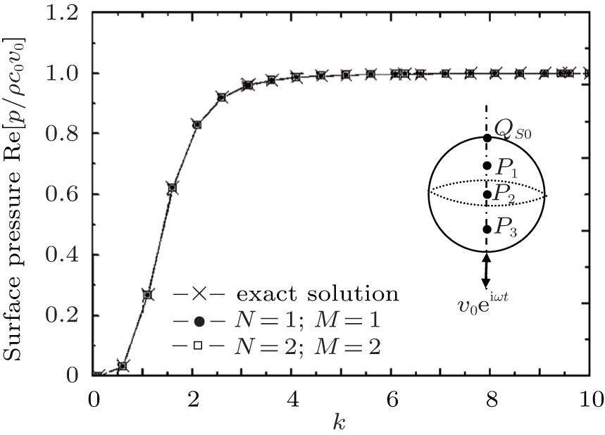
As a preliminary check of the accuracy of the multi-point multipole method described in this paper, one can take a pulsating sphere as the first case, of which radius R oscillates with a uniform radial velocity v0. The analytical solution of the acoustic pressure at the position Qs0(r, θ , z) radiated by the sphere is written as[29]

where 
Adopting the method, p is expressed in Eq. (7), and the coupling condition turns into the following expression:
Letting L = 0 in Eq. (A2) and Eq. (A3), and substituting them into Eq. (17), the collocation equation for the coefficients
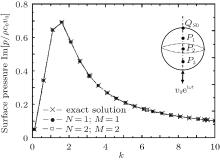
In Figs. 4 and 5, three virtual point sources are layered evenly along the radial line of the sphere with unit radius, and low (the third or sixth) order wave functions (i.e., N = 1, M = 1 or N = 2, M = 2) are truncated for each source point to obtain the real and imaginary parts of the acoustic pressure of point Qs0, which varies with wave number n. The numerical results are indicated to adequately coincide with the analytical one from these two figures for all the wave numbers.
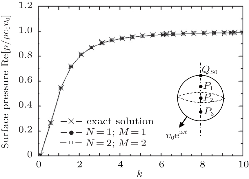 | Fig. 4. Real part of surface pressure of a pulsating sphere. |
 | Fig. 5. Imaginary part of surface pressure of a pulsating sphere. |
In fact, in the practical numerical simulation process, one can find that increasing the truncated number of the wave functions of the source points can enhance the accuracy of the numerical results. No more numerical examples are given for the limitation of this paper.
The next example is given for an oscillating sphere of radius R with a normal velocity v0 cosφ , where φ is the angle between the radial direction vector and the velocity one. The analytical solution of the acoustic pressure of point Qs0 (r, θ , z) radiated from the sphere can be described as[29]
In this example, the coupling condition can be written in a similar form to Eq. (17) by replacing v0 with v0 cosφ .
Figures 6 and 7 reveal the real and imaginary parts of the acoustic pressure for the point Qs0, which are obtained by the presented method and the analytical method respectively. Obviously, the method proposed in this paper is proved to be accurate once again.
 | Fig. 6. Real part of surface pressure of an oscillating sphere. |
 | Fig. 7. Imaginary part of surface pressure of an oscillating sphere. |
As mentioned in the introduction, when the geometric shape for the vibration structure deviates from a sphere, the convergence of the virtual source simulation method might turn poor. Hence, in this section, the last example is demonstrated for the acoustic radiation from a submerged stiffened cylindrical shell by applying the presented method compared with that in Refs. [30] and [31].
In order to compare the presented method with the one applied in Refs. [30] and [31] conveniently, the geometric parameters for the shell and the fluid are chosen to be the same as the ones given in Refs. [30] and [31]. Similarly, a unit concentrated external harmonic excitation with the excited frequency 6300 Hz is loaded on the surface of the shell at x = L/2, r = 0.2 m, θ = 0° . The Fourier series expansion in the circumferential direction of the external excitation is truncated with 26 terms to simulate the acoustic radiation field, i.e., the external excitation is expressed as follows:

in which, [30]
The ring ribs attached to the cylindrical shell can be considered as a point load acting at the location of the ribs. The details can be found in Ref. [30]. The observing points are located at a ring circle rotating around the cylindrical shell with x = L/2, r = 2 m through different observing angles.
The SPL for the acoustic radiation of the shell by using different methods is listed in Table 1. It displays that the SPL by using the presented method is approximate to the one by applying the experimental method. Meanwhile, compared with the SPL by applying the numerical method mentioned in Ref. [31], the one achieved by the presented method is more approximate to the experimental one.
| Table 1. SPLs for a submerged stiffened cylindrical shell with different methods. |
From the above numerical examples, one can find that the multi-point multipole method could be implemented to deal with the acoustic radiation problem for other cylindrical shells.
Meanwhile, it is worth pointing out that all the wave functions expressed in Eq. (8), chosen in the above examples, are truncated with a low-order one due to their superior performance to the higher order one when dealing with differentiation and summation manipulation. Hence, to simplify the computation of the sound pressure, the highest degree for the wave functions, i.e., N is chosen to be zero, and the highest order for the wave functions, i.e., M is chosen to be as small as possible in the following numerical examples. Additionally, to guarantee the accurate precision, the value of M should be ensured to be as big as possible. It is dependent on the number of the virtual point sound sources, i.e., NP. Hence, in the following section, a discussion would be carried out on the truncation of these wave functions series.
Considering the radiation SPL for an underwater ACLD cylindrical simply-supported at the two ends, for which the geometric and physical parameters are listed in Table 2, SPLs of the point Q0 (its coordinate has been given in Section 3) with different highest orders for the wave function (i.e. M) depending on the number of the virtual point source (i.e., NP) are displayed in Table 3.
In this case, kd = 1× 10⁶. A unit concentrated external harmonic excitation with the excited frequency 1000 Hz is loaded on the surface of the shell at x = L/2, r = R, θ = 0° . Meanwhile, only six different small values for M are listed.
From Table 3 it is revealed that when the number of the distributed virtual point sources tend to 13, the SPL of Q0 is convergent to about 126 dB, even though the value of M is chosen to be a smallest one, which means that much more virtual point sources can enhance the accuracy of the result. However, more virtual point sources will consume more of the computational source. Thus, one should increase the value of M to make up for the disadvantage of the less virtual point source. From Table 3, it could be found that when M tends to 4, 9 virtual point sources are sufficient enough to achieve the precise result. In order to ensure the precise and efficiency of the computation simultaneously, in this case, NP andM are chosen to be 8 and 4 respectively.
Unless otherwise stated, in the following numerical examples, the wave function series is truncated in the same way.
| Table 2. Geometric and physical parameters of a cylindrical shell treated with ACLD. |
| Table 3. SPLs of Q0 with different values of M dependent on the value of NP under the unit concentrated external harmonic excitation. |
A major goal of this paper is to analyze the parameter influence of the ACLD treatment on the acoustic radiation from cylindrical shells, so the cylindrical shells with different parameters of ACLD are further demonstrated in the following. All the geometric and physical parameters remain the same as the ones listed in Table 1 unless otherwise stated.
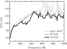
Firstly, different SPL spectrum curves given for the shell with two kinds of boundary conditions are shown in Figs. 8 and 9 respectively, showing that different link conditions between the shell and the rigid baffles bring a significant deviation to the SPL in the external acoustic field. At some frequencies the gap of the peak values for the SPLs is even up to almost 10dB. Moreover, as a whole, the SPL for the shell with a clamped boundary condition is lower than the simplysupported one. The reason might be that more vibration energies would be dissipated when the link condition of the two ends is clamped than being simply-supported. That is to say, it could be stated that a significant error might emerge when considering the link condition between the shell and the rigid baffles of the finite length cylindrical shell model as being simplysupported, which is widely adopted in much of the available literature.[9− 14]
Meanwhile, compared with the bare shell, the PCLD shell reduces the acoustic radiation much more especially at high frequency. At some resonant frequencies, the SPL could be reduced about 40 dB, which can make a considerable improvement in the stealth of submerged structure. Additionally, in a range from 0 Hz to 1000 Hz, the ACLD shell has a better suppression performance than the PCLD one. The SPL gap between the two treatments could be about 8 dB at some resonant frequencies. In this case, the feedback gain coefficient kd = 1 × 10⁶, which stays unchangeable in the following examples unless otherwise stated. Furthermore, thevboundary condition is always clamped-clamped for the following examples.
 | Fig. 8. Different SPL curves for three kinds of shells with simply supported boundary conditions at two ends. |
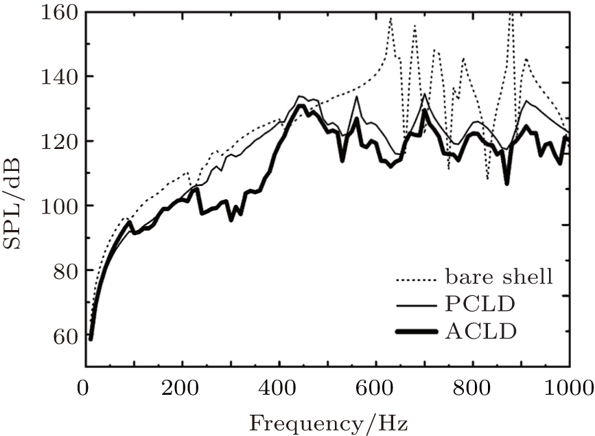 | Fig. 9. Different SPL curves for three kinds of shells with clamped boundary conditions at two ends. |
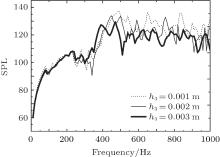
Then, the SPL curves with different thickness values of the piezoelectric layer are shown in Fig. 10. In general, when a thicker piezoelectric layer is treated on the shell, much more additional mass would be brought to the whole shell on the one hand. So better damping behavior can be found, which would be favorable for the sound reduction. But at the same time, active control force vector FV tends to be smaller on the other hand, which means that a negative influence on the sound suppression will be produced as well. Nevertheless, for the case described in Fig. 10, the positive influence is dominant. Hence, a thicker piezoelectric layer achieves better attenuation of the acoustic pressure to a large extent. Certainly, it is inevitable that a negative phenomenon appears at some frequencies. For example, in a frequency range from 250 Hz to 400 Hz, the value of the SPL is about 5 dB higher for the case with h3 being equal to 0.003 m than the one with h3 being equal to 0.002 m.
 | Fig. 10. SPL curves for ACLD shells with different thickness values of piezoelectric layer. |
Similarly, a thicker viscoelastic layer can enhance the damping performance of the whole system. However, a negative damping effect could also occur since the active control force caused by the piezoelectric layer is weakened indirectly when the sound wave passes through the viscoelastic layer to the base shell. Figure 11 shows three SPL curves for three kinds of thickness values of the viscoelastic layer. It can be seen that with the increase of h2, the damping effect remains worse at low frequency; however, it first turns better, then becomes worse at some high frequency peaks, which can be declared clearly from the SPL at a frequency around 450 Hz.
 | Fig. 11. SPL curves for ACLD shells with different thickness values of viscoelastic layer. |
In a word, when the thickness of the piezoelectric or viscoelastic layer for ACLD treatment, especially for the viscoelastic layer, is designed, the working frequency should be carefully investigated. When low frequency plays a major part in the working condition, thinner layers for ACLD should be the preferable choice, and vice versa.
Next, SPL curves with three different control gains are shown in Fig. 12. From which, less differences are revealed at the low frequency whereas better improvement is found at high frequency with increasing the value of kd. However, control gain always restricts the breakdown voltage of the piezoelectric layer. Meanwhile, a better damping effect is not always kept with kd getting bigger. For example, lower SPL is achieved for the case with kd = 1 × 10⁶ than the one with kd = 1 × 10⁸ at the peak frequency 907 Hz. Therefore, it is not an advisable choice to increase the control gain blindly in practical operation.
 | Fig. 12. SPL curves for ACLD shells with different gains of piezoelectric layer. |
Finally, in Fig. 13, coverage of the ACLD is discussed. A better damping effect can be described with the increase of coverage in general; however, as the coverage of ACLD exceeds 50%, superior suppression of the acoustic radiation pressure is not significant any more in the high frequency range. Furthermore, worse influence even occurs in the low frequency range. For example, the SPL with coverage 50% is lower with 8-dB difference than with the coverage 75% at some low frequency peak. After considering the cost of treatment together with its damping effect, the coverage of ACLD could be optimized further.
 | Fig. 13. SPL curves for different coverages of ACLD. |
Based on the previous research on the ACLD cylindrical shell without liquid, a series of first order integrated ordinary differential matrix equations in the frequency domain is presented in this paper. These matrix equations can be smoothly decoupled when the external excitation acting on the shell is harmonic and known.
By the internal source density simulation method, some virtual point sound sources are assumed to be distributed evenly along the axial line of the cylindrical shell to approach to the real external excitation. A superposition solution of the radiation acoustic pressure is explored with unknown coefficients by the method called the multi-point multipole method. Then, by the extended homogenous capacity integration method and superposition principles, the acoustic radiation of the cylindrical shell can be demonstrated in the paper by this method, which is proved to be available when discussing the acoustic radiation problems of a revolution cavity.
Numerical results of the SPL of the acoustic radiation from the shell with different parameters display that thicker thickness and larger velocity feedback gain for the piezoelectric layer, and larger coverage of the ACLD layer can obtain a better damping effect for the whole structure in general. Whereas, a thinner thickness for the viscoelastic layer is a better choice when lower frequency takes a major part in the working condition for the structure, and vice versa. Meanwhile, optimization should be carried out to achieve suitable values of these parameters at a minimum cost. And the presented method could be further developed for designing the real underwater structures combined with optimization methods.
Denote the coordinate of the source point Pk as (lPk, 0) (0 ≤ lPk ≤ L), the field point on the surface of cylindrical shell Qc as (xQc, R1) (0 ≤ xQc ≤ L)), and let xa = ω RPkQc/c0, xb = (xQc− lPk)/RPkQc, and 

Denote the coordinate of the point on the surface of the right rigid baffle QR as (L+ R1 sinβ , R1 cosβ ), let xaR = ω RPkQR/c0, xbR = (L+ R1 sinβ − lPk)/RPkQR, and 
Denote the coordinate of the point on the surface of the left rigid baffle QL as (− R1 sinγ , R1 cosγ ), and let xaL = ω RPkQL/c0, xbL = (− R1 sin γ − lPk)/RPkQL, and 

Substituting Eq. (14) into Eq. (13), after arrangement, one obtains
in which

Let
and choose Nc discrete field points along the meridian line of the cylindrical shell, denote the coordinates as ξ i = i/(Nc − 1), (i = 0, … , Nc − 1), then from Eqs. (9) and (A1), collocation equations for the points on the surface of cylindrical shell will be obtained as

where the sign sum(• ) represents the sum of vectors.
Similarly, choose NR discrete field points on the surface of the right semi-spherical rigid baffle, for which coordinate could be deduced from the discrete angle β i = iπ /2NR, (i = 1, … , NR) respectively, then from Eqs. (9) and (A2), collocation equations for the points on the surface of the right semi-spherical rigid baffle will be yielded as

Next, choose NL discrete field points on the surface of the left semi-spherical rigid baffle, for which the coordinate could be obtained from the discrete angle γ i = iπ /2NL, (i = 1, … , NL) respectively, then from Eqs. (9) and (A3), collocation equations for the points on the surface of the left semi-spherical rigid baffle will be obtained as

Till now, the whole collocation equations can be tidied up from Eqs. (B3)– (B5) as

The coefficients can be achieved from

| 1 |
|
| 2 |
|
| 3 |
|
| 4 |
|
| 5 |
|
| 6 |
|
| 7 |
|
| 8 |
|
| 9 |
|
| 10 |
|
| 11 |
|
| 12 |
|
| 13 |
|
| 14 |
|
| 15 |
|
| 16 |
|
| 17 |
|
| 18 |
|
| 19 |
|
| 20 |
|
| 21 |
|
| 22 |
|
| 23 |
|
| 24 |
|
| 25 |
|
| 26 |
|
| 27 |
|
| 28 |
|
| 29 |
|
| 30 |
|
| 31 |
|