


Analytical model for thermal lensing and spherical aberration in diode side-pumped Nd:YAG laser rod having Gaussian pump profile
[Moghtader Dindarlu M H† , Kavosh Tehrani M, Saghafifar H, Maleki A]
, Kavosh Tehrani M, Saghafifar H, Maleki A]
|
|


†Corresponding author. E-mail: elsa27m@gmail.com
In this paper, according to the temperature and strain distribution obtained by considering the Gaussian pump profile and dependence of physical properties on temperature, we derive an analytical model for refractive index variations of the diode side-pumped Nd:YAG laser rod. Then we evaluate this model by numerical solution and our maximum relative errors are 5% and 10% for variations caused by thermo–optical and thermo–mechanical effects; respectively. Finally, we present an analytical model for calculating the focal length of the thermal lens and spherical aberration. This model is evaluated by experimental results.
Side-pumped Nd:YAG laser rods have many advantages: they are simple, power scalable, reliable, and robust. A side-pump configuration is used to achieve high power lasers.[1] Since in this configuration the larger ratio of the laser crystal is pumped, it causes a strong thermal loading in the active material. Therefore the thermal effects such as thermal lens, thermally induced birefringence, and spherical aberration occur in the laser active material. Consequently, the losses in this configuration are very high for good beam quality operation.[2– 6] The thermally induced birefringence causes a significant decrease in output power and a marked change in beam shape.[1, 7] The thermal lens and the spherical aberration of the active medium affect the mode profile, the diffraction loss, the output average power, and other laser beam properties.[8– 11] Therefore a lot of methods have been used to compensate for the thermal effects.[12– 23] Usually to calculate the thermal effects of laser crystals, numerical finite element (FE) methods[24– 26] are used because the currently known analytical models are limited. The most important disadvantage of FE simulations is the time needed for making the calculations, as several minutes or even hours are needed; but the computation that uses an analytical model for the thermal effects takes only a few seconds. An additional advantage of analytical models is that the influence of various parameters can be analyzed directly by means of an explicit analytical expression. So far, many analytical models have been presented for thermal effects of the laser rod:[4– 6, 10, 27– 38] a large number of them are for the end-pumped configuration and only a few models are for a side-pumped laser rod. The thermal effect of the Nd:YAG laser rod is based on the temperature distribution. In the initial studies the temperature distribution had a parabolic shape due to the consideration of the homogeneous pump and temperature-independent physical parameters of the laser rod.[4, 10, 34, 37, 38] Thus, the refractive index variation had a second-order dependence on the radius of the rod, and the laser rod was optically equivalent to a perfect thick lens with two focal lengths. Therefore, there was no spherical aberration effect. As a result, thermal effects obtained in these studies cannot be completely comprehensive and accurate. The temperature distribution obtained from Ref. [2] had a fourth-order dependence of the radial coordinate. This led to the spherical aberration in addition to the thermal lensing effect.[2] However, for the calculations in this work, the thermal expansion coefficient was supposed to be constant. Moreover, the pump has a parabolic distribution. In Ref. [27], the dependence of physical parameters on temperature was considered, and thermal effects such as thermal lensing and spherical aberration were obtained for the laser rod. However, in Ref. [27] also, the pump distribution was considered as a parabolic profile with an inhomogeneous factor.
In this paper, we present, for the first time to the best of our knowledge, a new analytical model for thermal effects in the diode side-pumped Nd:YAG laser rod having a Gaussian pump profile. In our previous article, [39] a precise temperature distribution was obtained by considering the Gaussian pump profile and the temperature-dependent physical parameters of the laser rod. In this paper according to the temperature and strain distributions obtained from Ref. [39], and taking the temperature-dependent dn/dT into account, an analytical model for refractive index variations is presented, which includes variations caused by the thermo– optical and thermo– mechanical effects. Then, the precise analytical models are derived for the focal length of thermal lensing and spherical aberration. Our analytical model has several advantages over other models. First, the absorbed pump distribution in the laser rod is considered as a Gaussian profile (close to the case in reality). Second, the temperature dependence of the thermal conductivity and the coefficient of thermal expansion, the two most important parameters of a laser rod, are taken into account. Third, the change in the refractive index of the laser rod is obtained up to the fourth-order on the radial coordinate.
To calculate the thermal effects of the laser rod, the temperature and strain distributions are needed. We adopt the distributions obtained in Ref. [39].
In our previous article, [39] we considered temperature-dependent thermal conductivity and thermal expansion according to the following equation:

where K0 is the thermal conductivity at temperature, and T0 = 300 K and a, b, c, ξ are the constants. Then, we obtain the temperature distribution and strain components for the laser rod (in the cylindrical coordinate as shown in Fig. 1) as follows:[39]


where


Tp and Tc are temperatures at rod surface and rod center; respectively

In the above equations, R and r are the rod radius and radial coordinate, respectively; Pabs is absorbed power in the laser rod, η is the fraction of absorbed power converted into heat, L is the pump length, ω is the width of the Gaussian distribution, E is the elastic modulus, υ is the Poisson’ s ratio, α Tc = α (T = Tc) and 
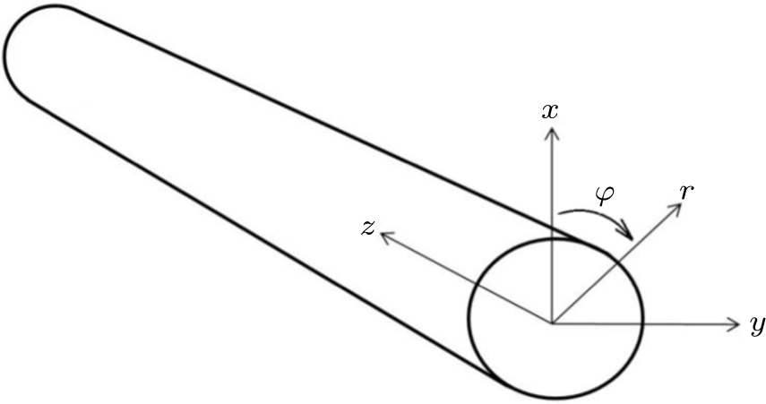 | Fig. 1. Rod geometry system in the cylindrical coordinate. |
| Table 1. Nd:YAG laser rod parameters. |
| Table 2. Numerical values of parameters. |
The refractive index gradients and strain occur in the laser rod due to non-uniformity of temperature. When the dependence of parameters such as dn/dT and the thermal expansion coefficient on temperature is considered, refractive index variation of the laser rod can be written as follows:[27]

where γ is responsible for the thermal lensing and Γ indicates the spherical aberration. These coefficients includes the thermo– mechanical (γ r, φ and Γ r, φ , where r represents the radial polarization, and φ denotes the tangential one) and thermo– optical (γ T and Γ T) effects, which are expressed as


Refractive index of the laser crystal varies directly with temperature, and this change is not linear, because dn/dT is not constant but varies with temperature.[27] We consider the refractive index variation with temperature up to the second-order, so one can write

where

and (d2n)/(dT2) are supposed to be constant around 300 K.[27] By substituting the temperature distribution Eqs. (3) into Eq. (16) and only considering the terms up to the fourth-order, we reach
According to Eqs. (13) and (17), γ T and Γ T can be expressed as
The strain matrix in cylindrical coordinates is defined as follows:[37]

where ε r, ε φ , and ε z are given by Eqs. (4)– (6). By strain and photo-elastic matrix, we can calculate the photo-elastic refractive index variation.[37] The strain matrix is given in cylindrical coordinates while the photo-elastic matrix is given in Cartesian coordinates (Eq. (21))[37]
The approximate values of the coefficients (P11, P12, and P44) are listed in Table 2.
Therefore, this calculation needs long coordinate conversions. The process is similar to that in Foster and Osterinks’ article.[37] Therefore, the details are not given, but they are summarized in Appendix A. Ultimately, according to calculations, the change in the components of the indicatrix will be the following
where Cr and Cφ are the usual birefringence coefficients, [37] and Qr, φ , 


Now the photoelastic refractive index variation for radial and tangential polarization (r, φ ) can be calculated by the following equation:[37]

According to Eqs. (22) and (28), we can write

Now γ r, φ and Γ r, φ are obtained by Eqs. (13) and (29) as


where N and M are given by Eqs. (9) and (10) and Cr, ϕ and 
According to the known coefficients, γ , i.e., γ r, ϕ and γ T, the focal length of thermal lensing can be calculated by the following equation:[27]

By considering the polarizations r, φ , this equation can be rewritten as follows:
where

By substituting Eqs. (18) and (30) into Eq. (34) and then inserting it into Eq. (33), the focal length of thermal lensing is calculated. Finally, we can consider the average focal length as the focal length of the thermal lens of the laser rod

Optical path difference (OPD) between the original wavefront and the aberrant wavefront was calculated[27]

where
Since the values of γ and Γ are different for the polarizations of r and φ , we can write

The coefficients of 

Therefore, by inserting Eqs. (19) and (31) into Eq. (39) and then inserting the resulting equation into Eq. (38), we can calculate the spherical aberration of the thermal lens. Under what has been given in Ref. [2], the spherical aberration is described as a radial dependence of focal length:
Now according to Eqs. (35) and (39), one can write

Using Eqs. (1), (2), (11), and (12) and the parameters listed in Tables 1 and 2, coefficients A, B, N, and M are obtained. Then, γ and Γ can be calculated by these coefficients and Eqs. (14), (15), (18), (19), (30), and (31). Finally, with γ and Γ and the calculation of ε (γ ) (Eq. (37)), the focal length (fr, φ ) and their variations are calculated according to Eqs. (32) and (41).
In order to provide theoretical results, we need to determine the numerical values of the parameters that appear in the equations of this paper, especially the physical characteristics of Nd:YAG. These parameters have different values. Efforts have been made to choose the best value for each of them. Values for the thermal conductivity at a temperature of 300 K vary from 9.7 W· m− 1· K− 1[40] to 14 W· m− 1· K− 1.[1] We choose the 10.5 W· m− 1· K− 1.[41] As for its dependence on temperature, we chose ξ = 0.7 because it was the best fit for the values of Refs. [42] and [43]. Values for dn/dT at 300 K also vary a lot: from 7 × 10− 6 K− 1[44] to 9.86 × 10− 6 K− 1.[45] We choose 9.86 × 10− 6 K− 1. For d2n/dT2 only two sets of values are available. They differ quite a lot: Nikogosyan’ s value is 2.5 × 10− 8 K− 2, [46] and Wynne’ s value is 3.8 × 10− 8 K− 2.[47] We use 3.8 × 10− 8 K− 2. The parameters of the Nd:YAG laser rod are listed in Table 1.
Since in Ref. [39] we showed that the profile of the absorbed pump power inside the three-side diode pumped rod is similar to a Gaussian profile, we introduce the same example as that given in Ref. [39] for evaluating the analytical model. A Nd:YAG laser rod with a length of 100 mm and a diameter of 3 mm is pumped from the side of the rod by diode laser arrays. This laser rod is placed in a glass tube with an inner diameter of 4 mm and an outer diameter of 5 mm. There is water flowing between the rod and the inner surface of the tube for cooling. The collection of the rod and tube is inside a reflector with a diameter of 14.5 mm. Laser diode arrays are put in front of three slits located on a reflective surface with a distance of 8.25 mm to the axis of the laser rod. The numerical values of parameters are listed in Table 2 for this example. A schematic cross section of the laser cavity for this example has been shown in Fig. 2.
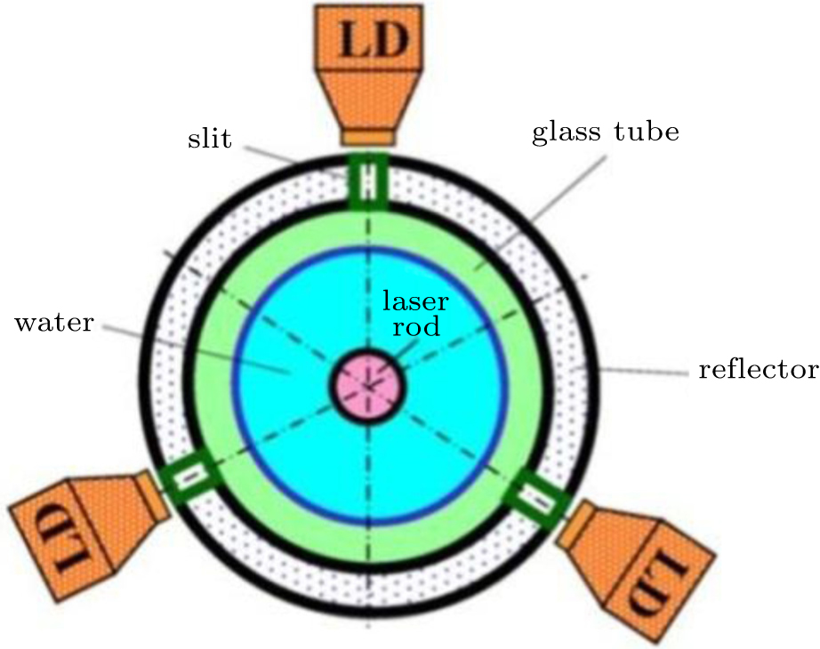 | Fig. 2. Schematic design relevant to the cross section of the laser cavity in the configuration of three-side pumping. |
In this section, we want to evaluate our analytical model for thermal lensing and spherical aberration. Because the focal length of the thermal lens, OPD, and spherical aberration are derived from refractive index variations (Eqs. (17) and (29)), it is sufficient for us to evaluate the refractive index variations.
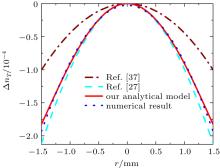
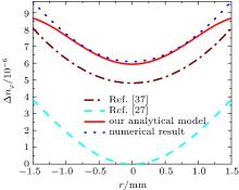
Since the numerical solutions are precise and reliable, we can use them to evaluate our analytical model. We numerically obtain the refractive index variations by numerical results given in Ref. [39] for temperature, stress, and strain distribution. The analytical and numerical results for refractive index variations are shown in Figs. 3– 5. In these figures, we also present the results obtained from Ref. [37] (where the homogeneous pump profile, temperature-independent thermal conductivity, and thermal expansion were considered) and Ref. [27] (where the parabolic pump profile, temperature-dependent thermal conductivity, and thermal expansion were considered). Now, with the existence of numerical results and those of Refs. [27] and [37], we can excellently evaluate our analytical model.
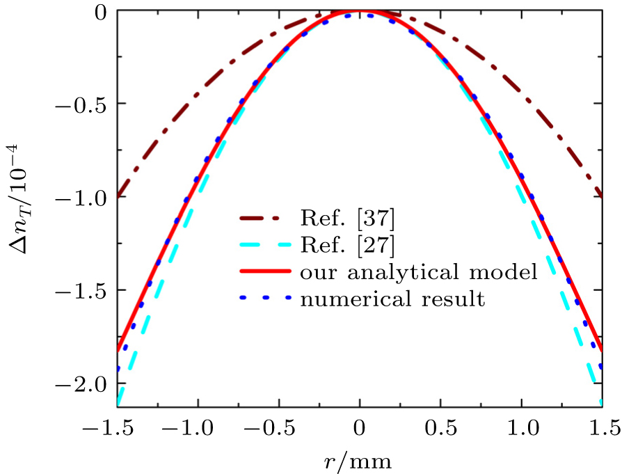 | Fig. 3. Refractive index variations caused by thermo– optical effects. |
 | Fig. 4. Variations of r component of refractive index caused by thermo– mechanical effects. |
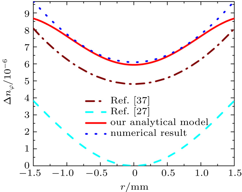 | Fig. 5. Variations of φ component of refractive index caused by thermo– mechanical effects. |
Figure 3 shows the refractive index variations caused by thermo– optical effects in the laser rod. It is apparent that the results from our analytical model are in better agreement with the numerical result when we compare maximum relative errors with the numerical results from our model and Refs. [27] and [37]. Maximum relative errors are 5% 10% and 48% for our model, Refs. [27] and [37], respectively in the rod surface. The refractive index variations caused by thermo– mechanical effects are shown in Figs. 4 and 5 for the r and φ component. According to Fig. 4, maximum relative errors with respect to the numerical result are 10%, 26% and 56% for our model, Refs. [27] and [37], respectively in the rod surface. Finally, according to Fig. 4, maximum relative errors with respect to the numerical result are 10%, 18% and 62% for our model, Refs. [37] and [27] respectively in the rod surface.
The values of errors show that the results from our analytical model (for refractive index variations) are in good agreement with the numerical results; therefore, the focal length of the thermal lens and spherical aberration obtained from refractive index variations will be reliable. Since in our analytical model, both the Gaussian absorbed pump distribution and the dependence of physical parameters on temperature are taken into account, this model is more precise than the previous one.
There are many formula for calculating the focal length of the thermal lens in the laser rod.[4, 27, 31, 38] Now for example as given in Subsection 3.2, we can compare the focal lengths obtained from these studies with those from our model (Eqs. (33) and (35)). The calculated values of focal length are listed in Table 3. Since our analytical model for refractive index variations is evaluated by numerical results (in the previous section), the focal length obtained from our model can be more reliable than from the previous studies.
| Table 3. Calculated focal lengths of thermal lens. |
Moreover, the focal length formula is presented in Refs. [10] and [36], which include the thermo– optical effects only. According to these studies, the focal length is calculated to be 53 mm and 56 mm for Refs. [36] and [10], respectively. As is well known, thermo– mechanical effects modify the focal length of the thermal lens by about 20%; [1] therefore, the focal length values of Refs. [10] and [36] may be mainly about 45 mm. According to Table 3, it is apparent that the focal length value in Ref. [27] is close to the value from our model. It can be due to considering the dependences of thermal conductivity and expansion coefficient on temperature.
In this section, we compare the spherical aberration results obtained from our analytical model with those from Refs. [10] and [27] for example given in Subsection 3.2. As mentioned before, spherical aberration can be shown as a radial dependence of the focal length or the refractive power of the thermal lens. We plot the refractive power of the thermal lens versus the radial coordinate in Fig. 6. According to Fig. 6, the values of refractive power difference are 0.4, 0.2, and 0.5 diopter for our model, from Refs. [27] and [10], respectively. It should be noted that the refractive power in Ref. [10] is only caused by the thermo– optical effect; while in our model and Ref. [27], the thermo– mechanical effects are also considered. Since the spherical aberration is extracted from the refractive index variation, the results from our model are reliable (because refractive index variations are evaluated by numerical results).
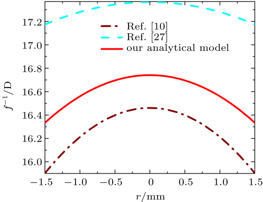 | Fig. 6. Radial dependences of the refractive power of thermal lens (spherical aberration). The unit 1 D = 1 m− 1. |
Another way to validate the analytical model is to compare its results with experimental results. In Ref. [27], the experimental values of focal lengths and spherical aberration have been obtained for the side diode-pumped Nd:YAG laser rod. The radius and length of the laser rod were 2.5 mm and 128 mm, respectively. The laser rod was pumped with powers of 1040 W, 1120 W, and 1200 W. The cooling temperature was 28 ° C. For this laser rod, we calculate the values of focal length (fr, φ ) and spherical aberration (OPDr, φ ) by our analytical model (Eqs. (33) and (38)). The calculated and experimental results for the focal lengths and spherical aberration are shown in Table 4.
| Table 4. Calculated and experimental results of focal lengths and spherical aberration for the side diode-pumped Nd:YAG laser rod (λ = 1064 nm). |
According to Table 4, calculated focal lengths and spherical aberrations are in good agreement with experimental results. The analytical model is reliable.
According tothe temperature and strain distribution obtained by considering the Gaussian pump profile and dependence of physical properties on temperature, we derive an analytical model for refractive index variations of the diode side-pumped Nd:YAG laser rod. Then this model is evaluated by a numerical solution and our maximum relative errors are 5% and 10% for variations caused by thermo– optical and thermo– mechanical effects respectively. Finally, an analytical model is presented for calculating the focal length of thermal lens and spherical aberration. This model is evaluated by experimental results. Therefore, for the knowledge of thermal effects in the side-pumped laser rod, we can use this analytical model instead of the numerical method, which needs a long time for calculations.
Firstly, we need a coordinate transformation matrix in which cylindrical coordinates in the direction of [111] transfer to the Cartesian coordinates in the direction of [100]. This matrix can be expressed as[37]
We will transfer the strain matrix (Eq. (20)) to the Cartesian coordinates [100] as follows:

We convert the matrix elements obtained in Cartesian coordinates into a column vector by using Nye’ s rule as follows:[48]
So the matrix ε ′ is converted to a column vector 

Now, according to the photo-elastic matrix (Eq. (21)) the variation of the indicatrix coefficients can be calculated by

Now we use Nye’ s rule again and this time we convert the column vector 

Matrix Δ B′ is in the Cartesian coordinates and we return it to the cylindrical coordinates with the following equation:

Finally, we can convert the matrix obtained from Eq. (A7) into a column vector by Nye’ s rule :

This vector will be as follows:
Since the light propagation is in the direction z the indicatrix components would be
According to the relevant component strain Eqs. (4)– (6) and the resulting matrix of these components we perform the calculations in accordance with the above steps and obtain the following results:
We can arrange the above equations and can write them as an equation in the form of

where the birefringence coefficients are defined as follows:

| 1 |
|
| 2 |
|
| 3 |
|
| 4 |
|
| 5 |
|
| 6 |
|
| 7 |
|
| 8 |
|
| 9 |
|
| 10 |
|
| 11 |
|
| 12 |
|
| 13 |
|
| 14 |
|
| 15 |
|
| 16 |
|
| 17 |
|
| 18 |
|
| 19 |
|
| 20 |
|
| 21 |
|
| 22 |
|
| 23 |
|
| 24 |
|
| 25 |
|
| 26 |
|
| 27 |
|
| 28 |
|
| 29 |
|
| 30 |
|
| 31 |
|
| 32 |
|
| 33 |
|
| 34 |
|
| 35 |
|
| 36 |
|
| 37 |
|
| 38 |
|
| 39 |
|
| 40 |
|
| 41 |
|
| 42 |
|
| 43 |
|
| 44 |
|
| 45 |
|
| 46 |
|
| 47 |
|
| 48 |
|