


Influence of a strong magnetic field on the hydrogen molecular ion using B-spline-type basis-sets
[Zhang Yue-Xia† , Zhang Xiao-Long]
, Zhang Xiao-Long]


†Corresponding author. E-mail: zyuex02@cqu.edu.cn
*Project supported by the National Natural Science Foundation of China (Grant No. 11204389) and the Natural Science Foundation Project of Chongqing (Grant Nos. CSTC2012jjA50015 and CSTC2012jjA00012).
As an improvement on our previous work [ J. Phys. B: At. Mol. Opt. Phys.45 085101 (2012)], an accurate method combining the spheroidal coordinates and B-spline basis is applied to study the ground state 1 σg and low excited states 1 σu, 1 πg,u,1 δg,u,2 σg of the
In our previous paper, [1] the one-center method is applied to study the ground state 1σ g and low-lying states 1σ u, 1π g, u, 1δ g, u, and 2σ g for the 
Obviously, the results in Ref. [1] are not sufficient for studying the influence of the magnetic fields for the chemical bond of the states of
The purpose of this paper is to optimize the method in Ref. [1] and Ref. [16] and investigate the influence of the magnetic field on the chemical bond. In this paper, the total energies and equilibrium distances of the ground states 1σ g, u, 1π g, u, 1δ g, u, 2σ g in all the field regions are recalculated. It is helpful for us to learn the advantage of the present method and narrow the gap between different methods. Next, the potential energy curves and the electronic probability density distributions of the states 1σ g, u, 1π g, u, 1δ g, u for a large region of B = 1, 10, 100, 1000 a.u. are plotted. Because the influence of the magnetic fields on the chemical bonds of the bound states and the antibonding states is different, so they are compared and discussed in detail.
As shown in Fig. 1, r1 and r2 represent the distances from the electron to proton 1 and proton 2, respectively, R is the internuclear distance, and there is a constant magnetic field along the z axis. The electronic Hamiltonian of 

where 

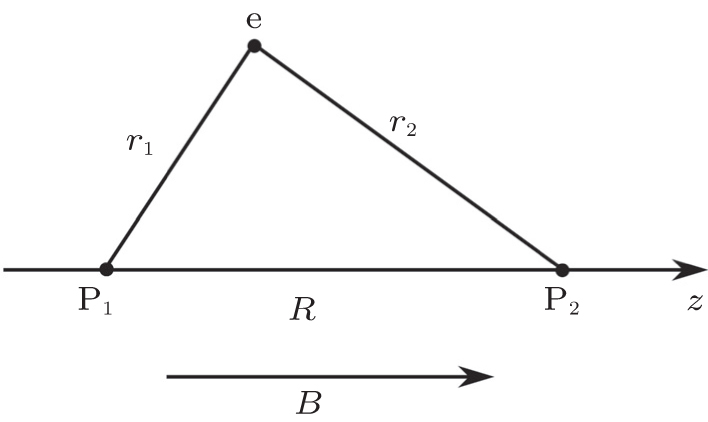 | Fig. 1. Model of the  |
In the case of a parallel magnetic field, the Hamiltonian of 


and

to replace r1 and r2 in Eq. (1), then the Hamiltonian for a given m in spheroidal coordinates can be read as follows:

with
and

being the kinetic, Coulomb interaction, and magnetic field terms, respectively. Comparing the HC term with that in spherical coordinates, which is

in Ref. [1], the expression in Eq. (3) is much more simple. In other words, the present method avoids the complicated numerical calculation on the singularities at the nuclear positions of 
The wavefunction of the system is expanded in symmetric B-spline type basis set as follows:[17, 18]
with

Here, ku and Nu denote the order and the number of B-spline basis function along the u axis. Similarly, kv and Nv along the v axis. π is the parity quantum number, and π = ± 1 represent even and odd states, respectively. It is worth mentioning that only half of the basis set is needed using the symmetric form in Eq. (5) comparing with the general B-spline basis in Ref. [19]. It is a very effective way to reduce the amount of calculation and speed up the convergence in the present method.
In addition, a proper knot sequence is also important for speeding up the convergence. In this project, the u axis knot sequence {uk} can be written as follows:

The knots in the domain [1, umax] are distributed exponentially as follows:
Here, subscript i values from [1, Nu − ku + 1] and α is an adjustable parameter.
The v axis knot sequence {vj} can be written as follows:

The knot distribution in the domain [− 1, 1] is regarded as a cosine function with

The knot distribution using the cosine function is more effective for speeding up the convergence than that in Ref. [16], where it is uniform. For example the 1π g state at B = 1 a.u. shown in the following Table 4, 80 × 60(Nu × Nv) basis is needed in Ref. [16], while 60 × 40(Nu × Nv) basis is enough to obtain the same results in this paper. For more detailed discussions about the knots and the properties of B-splines, readers can refer to Refs. [1], [20]– [23]. The eigenvalues and the corresponding wave functions of electronic states are obtained by diagonalization of the effective Hamiltonian (2) in a space spanned by the basis functions (4).
In the following, the equilibrium distances and total energies for the states 1σ g, u, 1π g, u, 1δ g, u, and 2σ g of 
Table 1 lists the equilibrium distances Req and total energies ET for the ground state 1σ g of 

Table 1. The equilibrium distances Req and total energies ET for the ground state 1σ g of  |
As shown in Table 1, the equilibrium distances Req and the total energies ET for the 1σ u state in magnetic fields with different strengths are listed in Table 2. Most of the calculations on the 1σ u state are concentrated on the domain B ≤ 1010 Gs as shown in Table 2. For the cases of B > 1010 Gs, there are two calculations, i.e., one by Turbiner[12, 13] and the other by us using the one-center method, [1] available. In the same way as in the case of 1σ g, the calculated equilibrium distances and total energies of the state 1σ u in the present method are closer to the data listed by Guan[3, 24] for 109 Gs≤ B ≤ 1010 Gs and Vincke at B = 2.35 × 10⁹ Gs than those obtained in the one-center method.[1] Results in the present method agree with the last digit given by Guan and Vincke. For 2.35 × 10¹⁰ Gs≤ B ≤ 1013 Gs, the results are closer to the data obtained by us in the one-center method[1] than Turbiner, [11] including the equilibrium distance and the total energy at B = 2.35 × 10¹⁰ Gs, where there is a larger difference between them. For the equilibrium distance from B = 2.35 × 10¹³ Gs, our data 2.143 is closer in agreement with 2.134 given by Turbiner than 2.02 by the one-center method. Also for B = 4.414 × 10¹³ Gs, there are no data available using the one-center method. However, the results of the present method are in good agreement with Turbiner’ s; this shows that this method is more suitable for 
| Table 2. Equilibrium distances Req and total energies ET for the excited state 1σ u. |
Comparing the numbers of the basis (Nu × Nv) for 1σ u and 1σ g, the amount of computation for 1σ u increases obviously; this may refer to the antibonding behavior of the 1σ u state. It can also explain why less works are found for the 1σ u state than the 1σ g state. Table 2 also shows the equilibrium distances Req decreasing and total energies ET of the 1σ u state increasing as the magnetic field grows from 109 Gs to 4.414 × 10¹³ Gs.
We compared the equilibrium distances Req and total energies ET for the excited state 1π u using different methods within a magnetic field ranging from 109 Gs to 4.414 × 10¹³ Gs as shown in Table 3. The present results are in perfect agreement with the data obtained by Guan in Refs. [3] and [24], Vincke in Ref. [11], and us using the one-center method in Ref. [1]. Even for B = 4.414 × 10¹³ Gs, the results of the present method are very consistent with those in the one-center method. Turbiner also gave the equilibrium distances Req and total energies ET with the field strength from 109 Gs to 4.414 × 10¹³ Gs. Their values are less accurate, but they are also closely consistent with our data.
We compare the energies of the 1π u state in Table 3 with those of the 1σ u state in Table 2, and the energy crossing is implied in the range 1012 Gs< B < 2.35 × 10¹² Gs.
In Table 4, the results of the antibonding state 1π g in different literatures are listed. The equilibrium distances of the 1π g were found to be larger than those of the antibonding state 1σ u. As shown in Table 4, most works focus on the case for B = 2.35 × 10⁹ Gs. Compared with the high-precision results given by Vincke in Ref. [8], the equilibrium distance is in agreement within 5 s.d. and the total energy within 11 s.d. For B = 109 Gs, the equilibrium distances listed in Ref. [1] and Refs. [12] and [13] are 18.08 and 20.10, respectively. The result in the present paper is in good agreement with that using the one-center method in Ref. [1]. For 1010 Gs≤ B ≤ 2.35 × 10¹² Gs, two sets of data, i.e., ours using the one-center method and Turbiner’ s, can be used to compare. The equilibrium distances and the total energies in the present paper are closer to those obtained by the one-center method. The accuracy of the equilibrium distance is estimated at about 3∼ 4 s.d. and the total energy at about 7∼ 8 s.d. For 1013 Gs≤ B ≤ 4.414 × 10¹³ Gs, only Turbiner’ s data are available. They are also closely consistent with ours.
| Table 3. Equilibrium distances Req and total energies ET for the excited state 1π u. |
In Table 5, the equilibrium distances Req and total energies ET for the excited state 1δ g in strong magnetic fields are compared with the results in other literatures. Two sets of results, i.e., Turbiner’ s and ours obtained by using the one-centermethod, can be found in various magnetic fields. They agree with each other very well, especially the present results and those obtained by the one-center method, where the equilibrium distances are consistent within 3∼ 5 s.d. and the total energies within 6∼ 9 s.d., except the case for B = 2.35 × 10¹² Gs. For the equilibrium distance at B = 2.35 × 10¹² Gs, the present data 0.3533 is closer to Turbiner’ s 0.353 in Refs. [12] and [13] than 0.3522 obtained by the one-center method in Ref. [1].
| Table 4. Equilibrium distances Req and total energies ET for the excited state 1π g. |
We compared the energies of the 1δ g state to those of the 1σ u state and 1π g state. Two energy crossings are found, one is between the states 1δ g and 1π g in the range from 2.35 × 10¹⁰ Gs to 1011 Gs, and the other between the states 1δ g and 1σ u in the range from 1013 Gs to 2.35 × 10¹³ Gs.
This is another antibonding state of the 
| Table 5. Equilibrium distances Req and total energies ET for the excited state 1δ g. |
| Table 6. Equilibrium distances Req and total energies ET for the excited state 1δ u. |
Comparing the 1δ u state in Table 4 and the 1π u state in Table 3 at the same magnetic field strength, the equilibrium distances of the 1δ u state are larger than the 1π g state by using the present method. It is different with Turbiner’ s conclusion, where for 1013 Gs≤ B ≤ 4.414 × 10¹³ Gs, the equilibrium distances of the 1δ u state are smaller than those of the 1π g state.
In Table 7, the results of the first excited state 2σ g for m = 0 and even parity series are listed. The equilibrium distance of the 2σ g state is larger than that of the ground state 1σ g. Far less investigation of this state in the 1σ g can be found in the literature. Only Turbiner and our group used the one-center method for all magnetic fields from 109 Gs to 4.414 × 10¹³ Gs and Kappes for B = 2.35 × 10⁹ Gs to investigate this state. The results obtained using different methods are consistent with each other. For example, for 109 Gs≤ B ≤ 1010 Gs, the present equilibrium distances coincide exactly with the results obtained by the one-center method in Ref. [1] and the energies are in agreement with 5∼ 6 s.d. However, present equilibrium distances and total energies at B = 2.35 × 10¹³ Gs and 4.414 × 10¹³ Gs are closer to the data of Turbiner. On the other hand, the one-center method shows weakness while the magnetic field strength is very high, similar to the case of the other antibonding states 1σ u, 1π g, and 1δ u.
| Table 7. Equilibrium distances Req and total energies ET for the excited state 2σ g. |
We compared the energies of the 2σ g state in Table 7 to those of the 1δ u state in Table 6 and the 1δ g state in Table 5. The two energies were found to cross within the range 109 Gs< B < 2.35 × 10⁹ Gs.
To analyze the influence of the different magnetic fields strengths on the 
 | Fig. 2. The Pecs of the states 1σ g, u of the  |
 | Fig. 3. The Pecs of the states 1π g, u of the  |
 | Fig. 4. The Pecs of the states 1δ g, u of the  |
Let us first consider the PECs of the bound states, that is, 1σ g, 1π u, and 1δ g in different magnetic field strengths. A common feature can be easily found. With increasing field strength, the more pronounced potential well located corresponding equilibrium distance is shown. It means stronger attraction exists with increasing magnetic field strength. The depths of the potential well are also given quantitatively by the dissociation energies of Table 8. As expected, for every bound state, the dissociation energies increase with the fields strengths from 1 a.u. to 1000 a.u. If we estimate the influence of the magnetic field on the state according to the ratio of the dissociation energies ED(B)/ED(B = 1 a.u.), they are 2.97, 9.43, 25.9 for the state 1σ g in B = 10, 100, 1000 a.u., respectively. The ratios are 4.24, 15.2, and 45.4 for 1π u and 4.58, 17.2, and 53.3 for 1δ g. For the same magnetic field strength, the ratios of the three states 1σ g, 1π u, and 1δ g increase, such as for B = 1000 a.u., 25.9 < 45.4 < 53.3. It shows the influence of the magnetic field increases with | m| from 0 to 2.
Next, let us take a look at the influence of the magnetic field on the antibonding states 1σ u, 1π g, and 1δ u. As depicted in dotted lines in Fig. 2#cod#x2013; Fig. 4, a shallow potential well exists in the PECs. The depths of the potential wells, that is, the dissociation energies of Table 8, are the order of magnitude of 10− 4 for B = 1 a.u. and 10− 3 for B > 1 a.u. Same as the case of the bound states, dissociation energies of every antibonding state increase with the increasing magnetic field strength from 1 a.u. to 1000 a.u. The ratios of the dissociation energies ED(B)/ED(B = 1 a.u.) are 3.13, 4.88, and 6.17 for 1σ u state in B = 10, 100, 1000 a.u., respectively, and they are 3.74, 5.97, 7.48 for 1π g and 4.23, 6.96, 8.85 for 1δ u. In the same way as in the case of the bound states, the ratios increase with increasing | m| for the same magnetic field strength. It means the same magnetic field strength has a greater influence on the state with larger | m| . For the case of the states with the same m and B, the radios are 25.9 and 6.17 for 1σ g and 1σ u with B = 1000 a.u., respectively. It is not difficult to find that the ratio of the antibonding state is much smaller than that of the corresponding bound state. The conclusion can be drawn that the same change of magnetic field strength has a smaller influence on the dissociation energies of the antibonding states than the corresponding bound states with the same m.
However, as we all known, existence of the potential well is not a criteria to judge whether a molecular bond is stable with respect to dissociation 
Table 8. Dissociation energies ED of the states 1σ g, u, 1π g, u, and 1δ g, u of    |
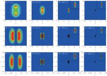
The EPDDs in the corresponding equilibrium distance Req in the x– z plane are plotted. The states from top to bottom are the bound states 1σ g, 1π u, and 1δ g in Fig. 5, and the antibonding states 1σ u, 1π g, and 1δ u in Fig. 6. The positions of the protons are labelled at the interaction points of the dotted lines along the x axis and the z axis. For every state, the density distributions for B = 1, 10, 100, 1000 a.u. are considered and compared from left to right in Fig. 5 and Fig. 6, which can better explain the change of the PECs with the magnetic fields strengths. For B = 100 a.u. and 1000 a.u., drawings of partial enlargement are placed at the upper right corner. We compare the density distributions of every state from left and right in Fig. 5 and Fig. 6, it is easy to find that the cylindrical symmetry is more obviously about the z axis with the increasing magnetic fields, and the electronic distribution is constricted in a smaller space. However, there is also different changing tendency between the bound states and the antibonding states.
First, let us discuss the change of the density distributions of the bound state 1σ g with the magnetic fields strengths. For B = 1 a.u. and 10 a.u., the electron is found with a great probability in the region around the two nuclei. When the | z | value between the two nuclei gets small, the probability becomes less and less and a saddle point appears at z = 0. When B is added to 100 a.u. and 1000 a.u., the saddle point disappears and a large density distribution of the electron occurs in the region between the two nuclei. The density distributions of the states 1π u and 1δ g are similar. A symmetrical density distribution occurs on both sides of the z axis for B = 1 a.u. With the magnetic field increasing from 1 a.u. to 1000 a.u., the distance of two regions gets closer to the internuclear axis. So for 1π u at B = 1000 a.u., the two regions come together. The electron can occur in the z axis with some probability. The density distribution is closer to the z axis and the increased probability between the two nuclei will screen and reduce the nucleus– nucleus repulsion. Thus, the bond length of the bound states of 
 | Fig. 5. The electronic probability density distributions of the bound states in the plane x– z in different magnetic fields. States from top to bottom are 1σ g, 1π u, and 1δ g. The drawings of partial enlargement are placed at the upper right corner. |
 | Fig. 6. The electronic probability density distributions of the antibonding states in the plane x– z in different magnetic fields. States from top to bottom are 1σ u, 1π g, and 1δ u. The drawings of partial enlargement are placed at the upper right corner. |
The EPDDs of the antibonding states are different from those of the bound states. For example, the density distribution for 1σ u in B = 1 a.u., mainly concentrate in the range of approximately − 1 < x < 1 and 4 < | z | < 6. There is a long range defined by − 4 < z < 4 between the two nuclei. No electron is found. The symmetrical distribution of the electron about the positions z = ± Req/2 shows the influence on the electron from the farther nucleus is a lot smaller than the nearer nucleus. With the magnetic field increasing, the distance of the two nuclei becomes shorter. Obviously the compression is the result of the effect of the magnetic field being greater than the repulsion between the two nuclei. It also shows that a stronger attraction occurs with the increasing magnetic field. However for B = 1000 a.u., the electronic distribution of positions z = ± Req/2 becomes asymmetric. It reflects that for B = 1000 a.u., the effect on the electron from the nucleus farther away cannot be ignored when the distance of the two nuclei is 2.848 a.u. The density distributions of the 1π g and 1δ u are similar. The electron mainly occurs in four regions of both sides of the z axis. With the magnetic field increasing, the region of the distribution is shrinking along the direction of parallel and perpendicular fields. For the state 1π g in B = 1000 a.u., these four regions of distribution merge into two around the z axis. Similar to the case of the 1σ u in B = 1000 a.u., the symmetry about the positions z = ± Req/2 is also destroyed because of the effect from the nucleus farther away. The similar effect is also found for the state 1δ g in B = 100 a.u. and 1000 a.u. The more significant asymmetry of the density distribution for the states 1σ u, 1π g, and 1δ u for B = 1000 a.u. shows the relative effect of the other nucleus farther away increases with larger | m| from 0 to 2.
In conclusion, we successfully applied the method combining the spheroidal coordinate and B-spline to calculate the equilibrium distances and the total energies of the states with | m| ≤ 2 of 

Further, the PECs and dissociation energies of the bound states and the anbibonding states for B = 1, 10, 100, 1000 a.u. show that the depth of the potential well increases with the increasing fields strengths. The stronger behavior of the attraction is reflected for a stronger magnetic field. Comparing the corresponding vibrational energies of the bound states in Refs. [12], [13] and [30], we can find that many vibrational states can exist in the potential wells of the bound states. It means the bound states 1σ g, 1π u, 1δ g are more stable in stronger magnetic fields. However, we cannot draw a conclusion on whether antibonding states can exist stably in strong fields due the accurate vibrational energies of the antibonding states. The increasing magnetic fields can cause the electron clouds to contract along both the parallel and perpendicular magnetic fields. However, the reason is different for the bound states and the antibonding states. For the bound states, EPDDs show that more and more electrons distribute in the region between the two nuclei with increasing magnetic fields. The screening of the two nuclear charges can explain the bond lengths decreasing with stronger fields strengths. For the antibonding states, the effect of the strong magnetic field is far greater than the Coulomb repulsion between the two nuclei, which is the reason why the bond length of the antibonding states decreases with the increasing magnetic field. With the distance between two nuclei closing, the electron is also influenced by the other nucleus farther away, and the symmetry of the electron clouds on the positions z = ± Req/2 changes. It is obvious for the EPDDs of the states 1σ u, 1π g for B = 1000 a.u. and 1δ g for B = 100, 1000 a.u. The asymmetry shows also that the influence of the nucleus farther away from the electron increases with larger | m| at the same magnetic field strength.
The present method can provide satisfactory results with a small amount of computation and save much computing time. The results we obtained in the present paper encourage us to extend the present method to study the influence of magnetic field strengths with different inclinations on the equilibrium distances, total energies, and molecular bonds of 
| 1 |
|
| 2 |
|
| 3 |
|
| 4 |
|
| 5 |
|
| 6 |
|
| 7 |
|
| 8 |
|
| 9 |
|
| 10 |
|
| 11 |
|
| 12 |
|
| 13 |
|
| 14 |
|
| 15 |
|
| 16 |
|
| 17 |
|
| 18 |
|
| 19 |
|
| 20 |
|
| 21 |
|
| 22 |
|
| 23 |
|
| 24 |
|
| 25 |
|
| 26 |
|
| 27 |
|
| 28 |
|
| 29 |
|
| 30 |
|
| 31 |
|