

The construction of general basis functions in reweighting ensemble dynamics simulations: Reproduce equilibrium distribution in complex systems from multiple short simulation trajectories
[Zhang Chuan-Biao, Li Ming, Zhou Xin† ]
]
]
|
|


†Corresponding author. E-mail: xzhou@ucas.ac.cn
*Project supported by the National Natural Science Foundation of China (Grant No. 11175250).
Ensemble simulations, which use multiple short independent trajectories from dispersive initial conformations, rather than a single long trajectory as used in traditional simulations, are expected to sample complex systems such as biomolecules much more efficiently. The re-weighted ensemble dynamics (RED) is designed to combine these short trajectories to reconstruct the global equilibrium distribution. In the RED, a number of conformational functions, named as basis functions, are applied to relate these trajectories to each other, then a detailed-balance-based linear equation is built, whose solution provides the weights of these trajectories in equilibrium distribution. Thus, the sufficient and efficient selection of basis functions is critical to the practical application of RED. Here, we review and present a few possible ways to generally construct basis functions for applying the RED in complex molecular systems. Especially, for systems with less priori knowledge, we could generally use the root mean squared deviation (RMSD) among conformations to split the whole conformational space into a set of cells, then use the RMSD-based-cell functions as basis functions. We demonstrate the application of the RED in typical systems, including a two-dimensional toy model, the lattice Potts model, and a short peptide system. The results indicate that the RED with the constructions of basis functions not only more efficiently sample the complex systems, but also provide a general way to understand the metastable structure of conformational space.
Exploring high-dimensional conformational spaces of complex molecular systems has long been the focus of computer simulation studies. Two challenges exist in this topic, how to thoroughly sample the conformational space, and how to understand the equilibrium (and dynamic) properties based on big simulation data. Although standard Monte-Carlo (MC) and molecular-dynamics (MD) simulation methods have been widely applied and achieved great successes, for many complex systems, such as glassy systems, phase-transition systems, and solvated biopolymers, sufficient sampling is by no means an easy task. With increased degrees of freedom, the potential energy landscapes of these systems are characterized by exponentially growing local energy minimums separated by energy barriers. Simulation trajectories are frequently trapped in small areas of this kind of rugged energy landscape, disproving the thorough exploration of the whole conformational space within limited simulation time. To overcome these difficulties, various advanced techniques beyond standard MD and MC methods have been developed, for instance, umbrella sampling[1] and its derivatives, [2, 3] J-walk, [4] multicanonical ensembles, [5] simulating tempering, [6, 7] conformational flooding, [8] hyperdynamics, [9– 11] parallel tempering, [12, 13] Wang– Landau sampling[14] and its derivatives, [15– 17] meta-dynamics, [18] multidimensional generalized-ensemble methods, [19] the integrated temperature method, [20] and the continuous temperature walking.[21] These methods can prominently accelerate the exploring in conformational spaces, while preserving the ability to reproduce equilibrium distributions.
Based on multiple parallel generated trajectories, the ensemble dynamics (ED) method[22– 24] provides an alternative way to further improve the ability of these (advanced) simulation techniques in sampling to bridge the gap between simulation ability and practical interest. Benefiting from the growing power of massively distributed computation, the ED method can reduce the wall-clock time required for data production. Actually, even in these advanced simulation methods, one does not exist which can guarantee to generate an ergodic trajectory within a reasonable time, it is usually necessary to generate a few trajectories starting from obvious different initial conformations then compare them. Thus, some knowledge-based order parameters are chosen to test the ergodicity, i.e., whether the distributions of these order parameters depend on the initial conformations. The low-dimensional test may suffer from the arbitrariness in the selection of order parameters, oversimplifying the description of systems.[25]
In the previous work, [26] we proposed a general method, which was previously denoted as weighted ensemble dynamics, now renamed as re-weighted ensemble dynamics (RED), attempting to overcome these challenges. The RED is based on multiple short MD (or MC) simulation trajectories, which start from dispersively-chosen initial conformations, and are generated under the same simulation condition (such as the same Hamiltonian, temperature, pressure, i.e., the same equations of motion). These trajectories may reach local equilibrium within a single metastable state, or transit among a few states. Although each single trajectory is too short to reach the global equilibrium, the whole set of trajectories may cover the conformational space, and could be combined to reproduce the equilibrium distribution.
The idea of combined analysis of parallel trajectories to reproduce global equilibrium distribution already exists, such as the weighted histogram analysis method (WHAM).[27] In the WHAM, the density of state of the simulation system is estimated by matching several different trajectories in their overlapping energy regions. The RED has a similar spirit to combine different trajectories based on their overlapping, in high-dimensional conformational space, rather than in onedimensional energy space as the WHAM. In the RED, we first define many conformational functions (named as basis functions) to sufficiently characterise the difference among trajectories, then design a systematical way to build the detailed balance among the visiting regions of these trajectories in the basis-function-spanned linear space. The global equilibrium distribution is then obtained.
In the RED, the sufficient and efficient selection of basis functions is a key.[28– 31] In a previous study, we usually chose the basis functions based on the physical intuition to the simulation systems. In complex molecular systems, such as protein, it is not a trivial task if we lack a priori and sufficient understanding on systems. It is very helpful to develop general ways to construct basis functions. In this paper, we focus on the question about a general construction of basis functions to describe complex molecular systems, then to combine many short trajectories together by the RED.
This paper is organized as follows. In Section 2, we present three methods on the construction of basis functions, and introduce the details by illustrating their applications in a two-dimensional toy model. In Section 3, we apply these methods in a short peptide and the lattice Potts model. In Section 4, we give conclusions and discuss the advantages and shortcomings of the methods. Details of the simulations are shown in Appendix.
The RED has been extensively described in the literatures.[26, 29] Here we give a brief overview to bring out the details of the new implementation.
Except for the possible effect of insufficient sampling, the difference between the conformational distribution of all the multiple short trajectories and the equilibrium distribution Peq(q) solely comes from the particular selection of the initial conformations, since every trajectory is generated by the same simulation algorithm that keeps the desired equilibrium distribution, only the initial conformations are different. Therefore, each conformation in the same trajectory should contribute equally to the final stationary property, but conformations in different trajectories may contribute to different weights. Then, the equilibrium ensemble average of any physical quantity A(q) is

where, wi is the weight of the i-th trajectory. 〈 · · · 〉 eq and 〈 · · · 〉 i denote the average over the equilibrium distribution and the i-th trajectory respectively.
The weight of the trajectory is determined by the deviation of the initial distribution from the equilibrium distribution, thus,

here Ω init, eq(q) ≡ Peq(q)/Pinit(q), and Pinit is the initial distribution, while qi0 is the initial confirmation of the ith trajectory. We can linearly expand Ω init, eq(q) by a complete set of conformational basis functions {Aμ (q)}

Here, A0(q) ≡ 1 is explicitly written out, and the basis functions are assumed to orthonormalize each other under the initial distribution, 〈 Aμ (q) Aν (q)〉 init = δ μ ν .
From Eqs. (2) and (3), we can obtain a self-consistent equation of wi,

where p is the number of trajectories, 〈 · 〉 i+ 〉 means the average in the initial part of trajectory i. Here we already set ∑ iwi = p without losing any generality.
Equation (4) could be rewritten as Gi · w = 0 with i = 1, … , p, and Gi = (Gi1, … , GiNt)T, which can be regarded as a vector mapped from the i-th trajectory. We can write a symmetric equation,

here, H = ∑ iGiGi is the variance-covariance matrix of the trajectory-mapped vectors {Gi}, with at least one zeroeigenvalue as the ground state of H, and the ground state eigenvector gives the weights of all trajectories for reconstructing the global equilibrium distribution.[26] By projecting the vectors, {Gi} to the H eigenvectors with zero (or near zero) eigenvalues, the trajectories are mapped into a lowdimensional space, where the non-transition trajectories inside different metastable states and the transition trajectories between these states can be identified easily.
In the RED, the selection of basis functions is crucial. The expansion in the RED require a complete set of basis functions in principle to guarantee the precision of Eq. (3), thus the number of basis functions is usually very large.
In this paper, we present three kinds of methods to construct basis functions.
(i) Various analytical physical quantities, such as dihedral angles, radius of gyration, distances of atom pairs, solvated energy, and helix probability, could be applied as basis functions.
(ii) Cell functions in the space spanned by the physical quantities. We split the physical quantity-spanned space into some discrete cells, and define cell functions as basis functions.
(iii) RMSD-based-cell functions. Using a technique similar to Markov state models, [32] we split the conformational space into overlapped cells based on RMSD (root mean square deviation) between conformations. The cells are then analyzed by principle component analysis (PCA) to get a set of orthogonal basis functions.
As described in the reference paper[20] and mentioned above, if we have enough priori knowledge about the system, we could use various analytical functions of some physical quantities as basis functions. To be specific, for a protein system, we could use dihedral angles, radius of gyration, distances of atom pairs, solvated energy, helix probability, and so on. We will employ this method to analyze a short peptide in Subsubsection 3.1.2.
For the space spanned by a few characteristic physical quantities of a system, we could split the space into many discrete cells, and define basis functions based on the cells. Below is the procedure to construct these basis functions.
a) Equally dividing each physical quantity into n bins, then we have nd grids in the space spanned by d quantities.
b) Collecting those grids containing sufficient sample conformations as cells. Empty grids are neglected, and some neighbouring grids with less sample points are merged into one cell. Each cell corresponds to a cell function, Cμ (q) = 1 if q is inside the μ cell, otherwise zero.
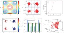
We first illustrate the method in a two-dimensional system. There are four major potential wells (I, II, III, and IV), shown in Fig. 1(a). 1500 simulation trajectories were generated at temperature 0.38 (in dimensionless unit). The initial position of every trajectory was randomly selected in the square region [− 2, 2] × [− 2, 2]. Each trajectory was simulated for 15 (in dimensionless time unit). More details are given in Appendix A. We select 600 trajectories from all the 1500 trajectories with a non-uniform initial distribution, 250, 50, 50, and 250 trajectories starting from state I, II, III, IV, respectively, to test the ability of the RED in reproducing the equilibrium distribution.
We split the conformational space (x, y) into uniform n × n grids, and apply the cell functions as basis functions. Here, n = 10, see Fig. 1(b).
There exists only one zero eigenvalue of the H-matrix under T = 0.38, see Fig. 1(c), suggesting that the equilibrium properties of the system could be reproduced with current simulation data. The obtained weights of trajectories are plotted in Fig. 1(d), trajectories start from state I and state III have the same weights, with a small fluctuation. This is consistent with our supposition, that is, the weight of a trajectory mainly depends on the state where the trajectory starts. For simplicity, we count the samples in every state, and plot the counted number in Fig. 1(e). Due to its biased initial distribution and the short simulation time, the obtained sample distribution is different from the equilibrium one. In contrast, the reconstructed distribution is very close to the theoretical expectation. Although the initial distribution is biased, the changing of the trajectory weights offset the bias, leading to the equilibrium distribution. In order to estimate the error of the reconstructed distribution, we repeat the RED analysis 100 times by choosing different simulation trajectories. The error bar is the standard deviation of these results.
We project {Gi} to the second, third, and fourth eigenvectors of H, which maps each trajectory i to the point 

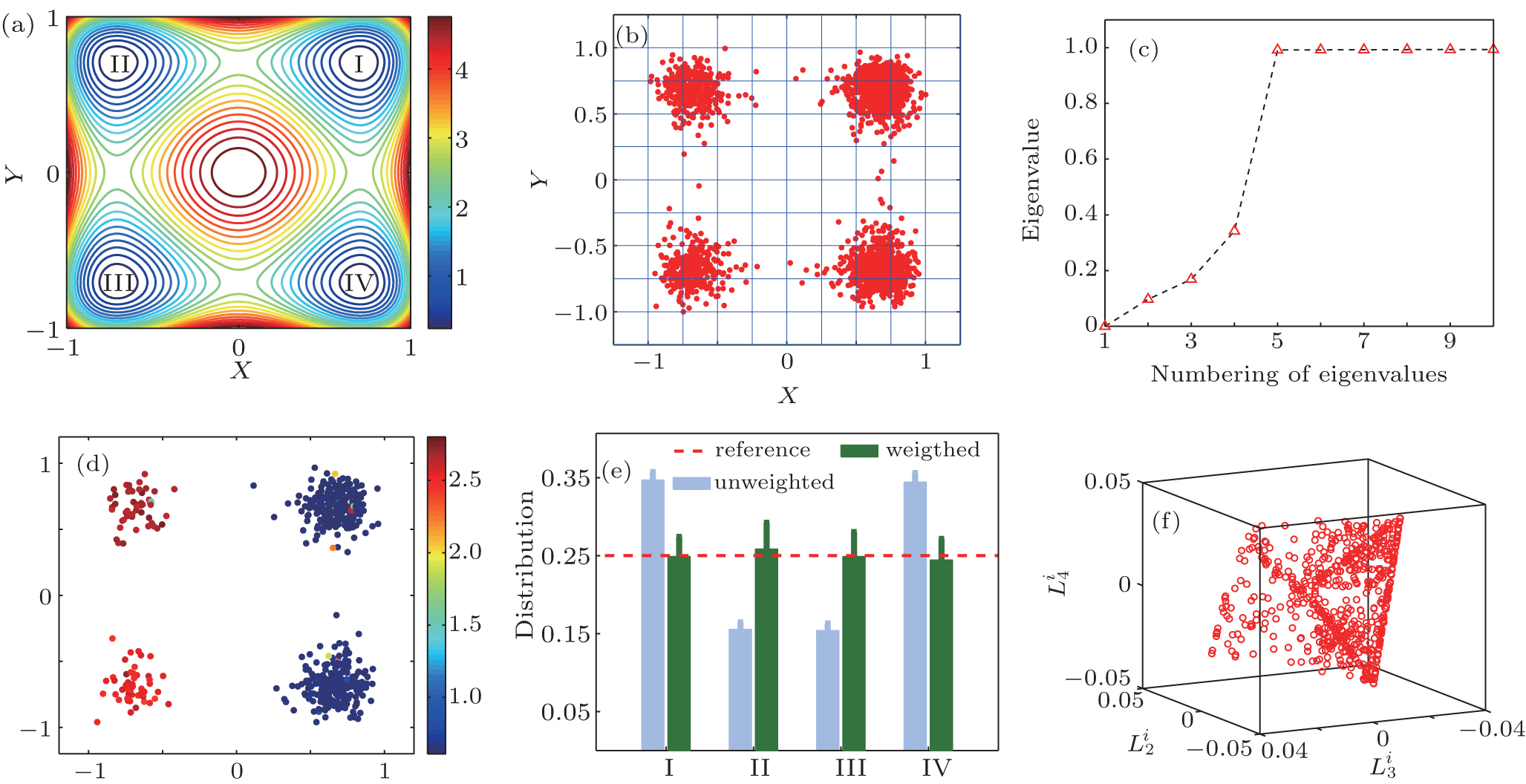 | Fig. 1. (a) The two-dimension-four-state potential energy surface. (b) Splitting conformational surface into 10 × 10 grid. (c) The first ten eigenvalues of the H matrix. (d) 600 colored dots are trajectory weights of the 600 trajectories. (e) Reconstructed distribution (green bar), original distribution (blue bar) and theoretical value (dash line). (f) The projection of {Gi} to the second, third, and fourth eigenvectors of H. |
Generally, it is possible to RMSD to split the sampled conformations into groups then construct basis functions. Here, RMSD is the measurement of the average distance between two conformations a and b,

where, n is the dimension of conformational vectors with the components, such as {ai} and {bi}. Basis functions could be constructed as follows.
a) Splitting Given a set of conformational samples, we randomly choose a conformation O1 in the set as a reference, then calculate RMSD between O1 and the other. The samples whose RMSD are smaller than a specified value 

b) Mapping Now any conformation sample S should be assigned to at least one cell, which is represented by vector {Ai(S)} with the index of cells, i = 1 … N
where, RMSD(S, Oi) denotes the RMSD between sample S and the center sample Oi of cell i.
c) PCA It should be noted that the overlapping among the cells is quite large. We can employ principle component analysis (PCA) to orthonormalize these cell functions to form a set of complete orthogonal basis functions.
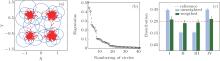
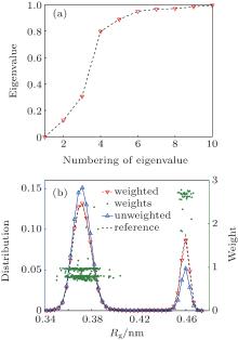
In the two-dimensional toy model (Subsubsection 2.2.2), RMSD between two samples is the geometrical distance between them. 41 cells are determined based on the RMSD matrix (Fig. 2(a)). Then, a two-dimensional coordinate (x, y) plane could be mapped onto 41-dimensional space (A1, … , An). As shown in Fig. 2(b), the first 36 eigenvalues account for over 90% of the sum of total eigenvalues. Thus, 36 corresponding eigenvectors are selected as basis functions. By using the RED, the reconstructed distribution is consistent with the theoretical value (Fig. 2(c)). Here, the number of cells is a tunable parameter. In this toy model system, actually, ten cells are sufficient to give good enough results (Fig. 8).
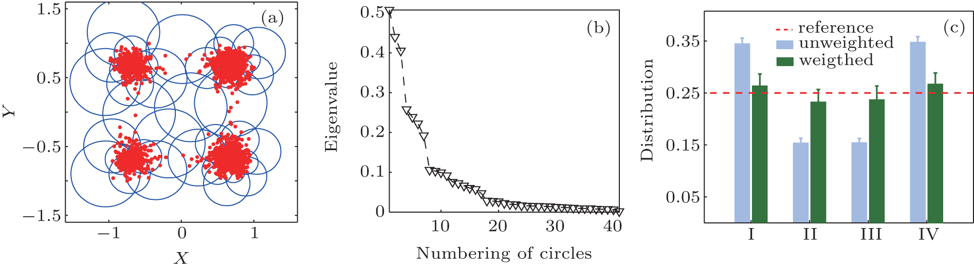 | Fig. 2. (a) The 41 cells are shown as the blue circle. (b) The 41 eigenvalues in PCA analysis of cells. (c) Reconstructed distribution (green bar), original distribution (blue bar), and theoretical value (dash line). |
In this section, we apply the above three methods on basis functions construction in two typical systems, the short peptide (Ace-(Gly)2-Pro-(Gly)3-Nme) and the lattice Potts model.
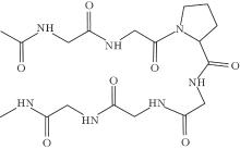
The molecular structure of the short peptide Ace-(Gly)2-Pro-(Gly)3-Nme is shown in Fig. 3. This molecular is hydrophobic and its hairpin conformation is unstable in a solvent; [33] we simulate the system in a vacuum. The radius of gyration of heavy atoms (Rg) is a well-known slow variable, which is relatively straightforward to manually identify metastable states and get the equilibrium distribution from a conventional dynamics simulation. According to previous studies, [31, 35] the free energy along Rg has a “ doubel-well” structure, respectively corresponding to a globular and a β -hairpin folded conformation. Here,

where mi is the mass of atom i and ri is the position of atom i with respect to the center of mass of the molecule, and the sum run over all atoms except hydrogen.
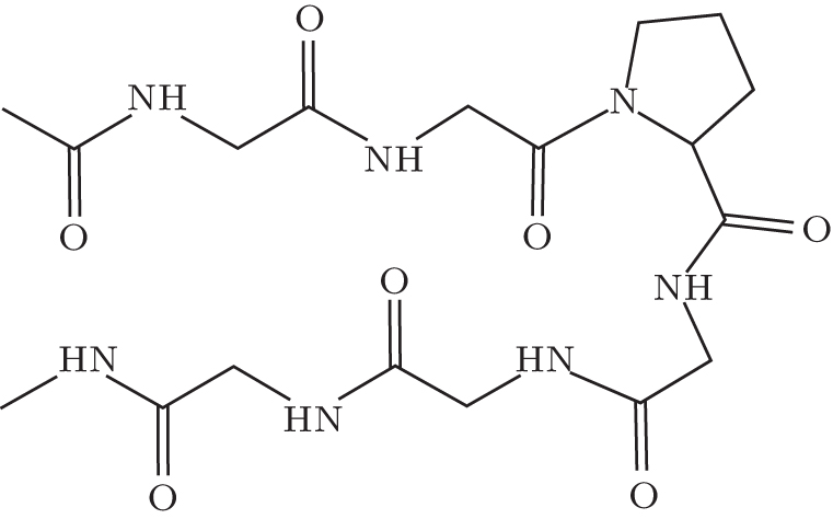 | Fig. 3. The Ace-(Gly)2-Pro-(Gly)3-Nme peptide in a β -hairpin conformation (sketch). |
(I) Simulation details
Initial configuration was generated using the PyMOL package. The MD data were obtained with the version 4.6.5 of the GROMACS simulation package[36] and Amber96 force field.[37] Simulations were carried out at 300 K using the v-rescale algorithm[38] with a 2-fs times step and τ T = 2 ps. The LINCS algorithm[39] was applied to all bonds for constraints. The peptide was run in a vacuum with 12 Å cutoff for the nonbonded interactions.
We first use method (iii) to construct basis functions. RMSD between two structures is
here, 
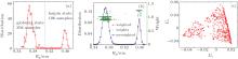
All 500 trajectories (400 ns) are used in the RED. The reconstructed distribution is shown in Fig. 4(b) (red line). The original distribution is very close to the reconstructed distribution, and the weights of trajectories are all around 1. It means that after 400 ns evolution, the system almost reaches equilibrium.
In order to verify the reliability of the RED, we only reserve the first 100 ns of every trajectory, and randomly discard 71 trajectories that started from the “ hairpin” state, then the remaining 429 100-ns trajectories (394 started from “ globular” and 35 from “ hairpin” ) are used in the RED. The distribution of raw data (non weighted) is shown in Fig. 5(b), which is very different from the equilibrium one. After the RED analysis, the weights of trajectories started from the hairpin are almost doubled, compared to previous results. As a consequence, the weighted distribution almost coincides with the reference distribution.
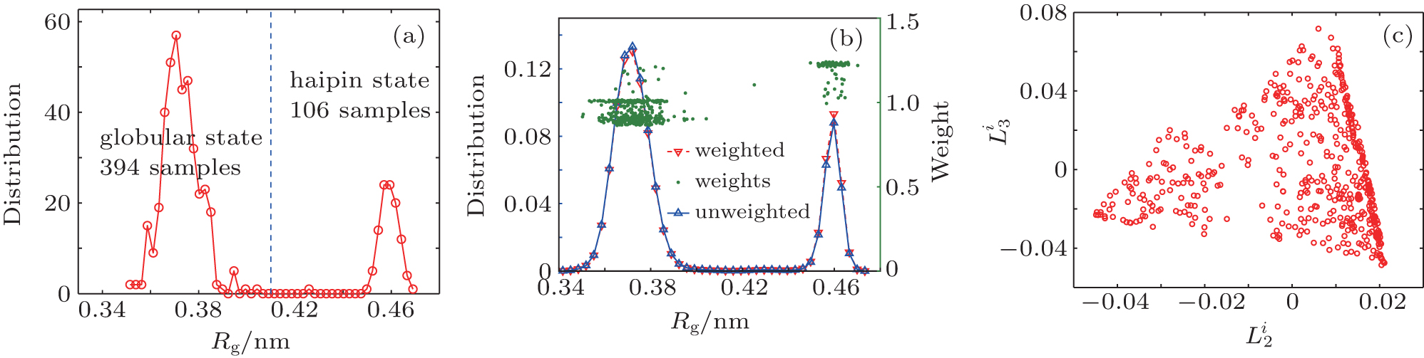 | Fig. 4. (a) The distribution of 500 initial conformations along the Rg axis. There are 394 trajectories starting from the globular state, and 106 trajectories from hairpin state. (b) The blue line is the original distribution. The red line is the weighted distribution. Green points are weights of all trajectories. (c) The projection of {Gi} to the second and third eigenvectors of H. |
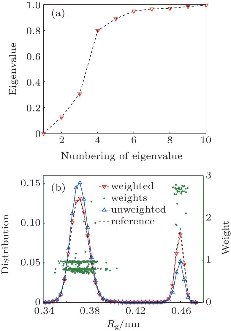 | Fig. 5. (a) The eigenvalues of H. (b) There are 394 trajectories starting from the globular state, and 35 trajectories from the hairpin state. After 100 ns simulation, the distribution is far from equilibrium (blue line), green points are weights of trajectories, and the reconstructed free energy profile (red line) closely matches the reference value (black line). |
We project {Gi} to the second and third eigenvectors of H. In the two-dimensional space, the 429 trajectories are shown as points in Fig. 4(c). All points together sketch out a triangle, which means there are three meta-states, rather than the two states reported in the previous studies.[34, 35] The conclusion of three states can be also found from the eigenvalue of H and the weights of trajectories. As shown in Fig. 5(a), there are ns = 2 eigenvalues significantly smaller than one, which implies that this system has three (ns + 1) metastable states. As shown in Fig. 5(b), the weights could be clustered into three clusters, corresponding to the three metastable states. By analyzing the conformations of these three states, we find that end-to-end distance (Dee) of heavy atoms should be included as a new order parameter, the “ globular” state has two substates with almost the same radius of gyration Rg, but very different end-to-end distance Dee. We plot the free-energy surface on the (Rg, Dee) plane in Fig. 6(a), then we can divide the whole conformational space into three states, A, B, and C, as shown in Fig. 6(a). There are 181 trajectories starting from state A, which looks like a helix, 213 trajectories from state B, a “ globular” state, and 106 trajectories from state C, the “ hairpin” state.
 | Fig. 6. (a) Free energy surface on Rg– Dee plane, this plane can divide into three parts corresponding to three metastable states. (b) The error of reconstruct distributions of three methods. Horizontal axis is the index of three states. Vertical axis is the deviation of reconstruct distributions from the reference distribution. |
(II) Comparison between three methods
In this subsection, we compare the performance of the three methods. Following the above procedure, we randomly discard 131 trajectories that started from region A, and analyze the remaining 369 (100 ns) trajectories based on three different basis function constructions.
First, six pairs ϕ – ψ of dihedral angles are used to construct basis functions by the method (i). The dihedral angles first need to be transformed to a linear metric coordinate space. This can be achieved by the transformation, [40]q2n− 1 = cosψ n, q2n = sinψ n, where n = 1, … , M and M is the total number dihedral angles. Here, M = 12, so there are total 24 basis functions. After getting the weights of trajectories, we count the samples in three states, and plot the deviation of weighted distributions from the reference distribution in Fig. 6(b) (red line). Second, physical quantity-based cell functions are used to calculate weights of trajectories (method II). To be specific, we divide the Rg– Dee plane into 100 equal grids. The deviation is shown as the cyan line in Fig. 6(b). Finally, we use the method (iii) to calculate the deviation between the RED results with the reference equilibrium distribution, which is shown as the green line in Fig. 6(b). It can be seen that all the three methods perform well for the short peptide system. For a system without enough priori knowledge, methods (ii) and (iii) might be better choices. More importantly, we could obtain a new order parameter to describe the system through analyzing the characteristics of conformations inside different states. Then we might use the order parameters to further enhance the sampling efficient, by using the advance simulation techniques, such as the umbrella sampling, [1] and metadynamics[18] simulation.
Potts model is a generalization of the Ising model, a model of interacting spins on a crystalline lattice. It is often used as a model system to discuss phase transition.[41] In this subsection, we use the RED to analyze the phase behaviour of the 2D Potts model. The Hamiltonian of the Potts model is defined as

where the summation is taken over all nearest neighboring pairs on the 2D lattice, each spin takes value qi = 1, … , Q and δ is the Kronecker delta. In the following, we set N = L2, L = 16, Q = 8, J = 1 and take the periodic boundary condition in the 2D lattice. RMSD between two conformations (a and b) is calculated as below:

here, 
We generated 900 trajectories starting from random initial conformations at T = 0.7455. The length of every trajectory is 2200 MC cycles (1 MC cycle = N spin varying steps). The first 200 MC cycles are regarded as the relaxation process. The eigenvalue of H is shown in Fig. 7(a). There are nine eigenvalues which are significantly smaller than one, meaning that this system has nine metastable states. We project {Gi} to the second, fourth, and sixth eigenvectors of H to form a three-dimensional (3D) space (Fig. 7(b)), and the eighth eigenvector of H is represented and visualized as different colors of points. In this (3 + 1)-dimensional space, the 900 trajectories can be clustered into nine clusters. We find that the mean value of q of each conformation, 

where Nmax = max(Ni) and Ni is the number of spins with the state qi. We project all conformations to the m– q̄ plane. Obviously, in the two-dimensional space (m, q̄ ) (Fig. 7(c)), the 2D-8 states Potts model can be divided into nine meta-states, one paramagnetic state corresponds to the bottom state in Fig. 7(a), and the top eight states correspond to the eight ≡ alent ferromagnetic states with different q value.
In order to get a reference distribution, eight long trajectories were simulated at T = 0.7455. The entire run of each trajectory is 1.2 × 10⁸ MC cycles. Then, we count the number of samples in each ferromagnetic state and show the results in Fig. 7(d). The distance between each red point and the original point correspond to the number of samples in each ferromagnetic state. As shown in the figure, the number of samples in eight states are roughly equal, which implies that the system reaches equilibrium. The eight green points that compose a regular octagon could be taken as a reference line.
We also construct biased initial distribution and reproduce the equilibrium distribution by the RED. Here, we use method (iii) to construct basis functions. At T = 0.7455, 2000 trajectories were generated, and all of them are 2.2 × 10³ MC cycles long. The first 200 MC cycles are regarded as the relaxation process. We randomly select (150, 50, 50, 150, 150, 50, 50, 150, 50) trajectories that started from the eight ferromagnetic states and the paramagnetic state, respectively. Therefore, the initial distribution of the selected trajectories is very different from the equilibrium one. After 2 × 10³ MC cycles, the system does not yet reach equilibrium due to the short simulation time(Fig. 7(e) (blue line)). There exists only one zero eigenvalue of H, suggesting that the weights of trajectories can be calculated to reproduce equilibrium. The weighted distribution is plotted in Fig. 7(e) (red line), which is consistent with the theoretical value (black line). Although each single trajectory is short and far from equilibrium, the equilibrium distribution can be correctly reproduced by the RED.
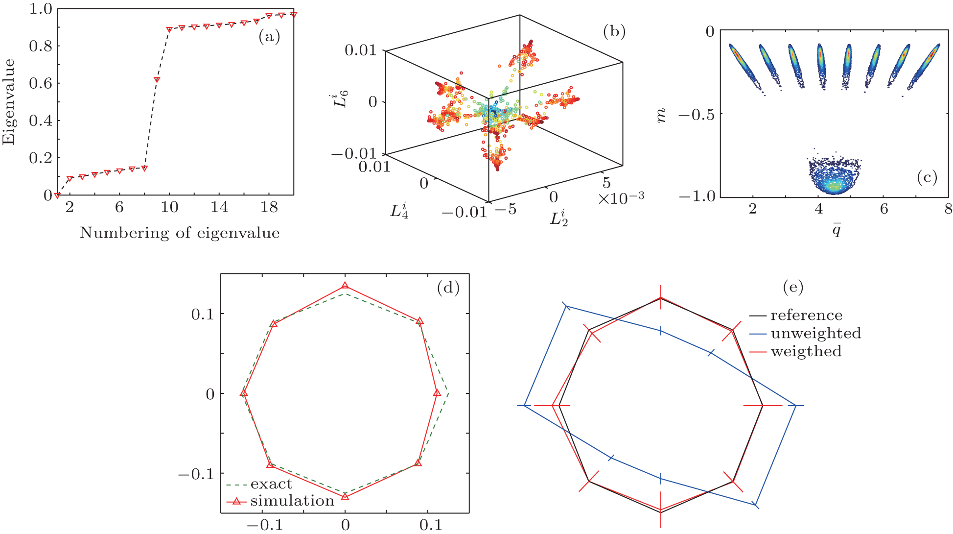 | Fig. 7. (a) The eigenvalues of H. (b) The projection of {Gi} to the second, fourth, and sixth eigenvectors of H, the color of points corresponding to the eighth eigenvectors of H. (c) In the two-dimensional space (m, q̄ ), the trajectories can be clustered into nine states, one paramagnetic state and eight ferromagnetic states. (d) The samples in eight ferromagnetic states are expressed through a radar graph: the blue line is calculated from the simulation data, while the red dash line is the reference value. (e) The samples distribution (blue triangles), reconstructed distribution (red triangles), and reference distribution (black line). |
The RED is expected to be an efficient way to enhance sampling and to explore conformational space of complex systems. The appropriate choice of basis functions is crucial to the practical application of the RED. In this paper, we present three methods for constructing basis functions. We may use the priori known important collective variables as basis functions, or split the collective variable spanned space into discrete cells, and define cell functions as basis functions. While lacking the knowledge of these collective variables, it might be a good way to use RMSD between conformations to divide conformational space into many small (partially overlapped) cells, and use the cell functions to construct a complete set of basis functions. We show the application of these methods in a two-dimensional toy model, the lattice Potts model, and the short peptide, Ace-(Gly)2-Pro-(Gly)3-Nme. All three methods could reconstruct the equilibrium distribution forming short trajectories well. Furthermore, new order parameters in the Potts model and short peptide are found through characterizing the difference of conformations inside the obtained metastable states.
For a protein with hundreds or more residues, long time scale conformational change may occur only at some specific sites, most residues just fluctuate around their equilibrium positions. In this situation, the global RMSD which is an average of the difference of all atoms between two conformations might be not a good parameter to distinguish two conformations that belong to different metastable states. The local RMSD which only measures the difference of partial atoms may be a better choice to construct basis functions. A more detailed discussion on this interesting and practical topic will be presented in our future work.
The over-dampened Langevin equations
were used to generate the simulation samples. A reflecting boundary condition was imposed. Here, γ is the frictional coefficient. kB is the Boltzmann constant, T is the simulation temperature, ɛ 1(t) and ɛ 2(t) are independent white noises satisfying with 〈 ξ (t)iξ (t′ )j〉 = δ (t − t′ )δ ij denoting the ensemble average of noise, while 〈 · · · 〉 denotes the ensemble average. We set kB and γ as unity to get the dimension-reduced units for time, position and temperature. The potential of the toy model U(x, y) was defined as
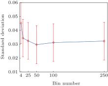
The basis functions number N is a free parameter in method (iii). Here, we discuss how to select N. In the two-dimensional model system the exact equilibrium distribution is uniform, the standard deviation of the distribution (std) measures the error of the reconstructed distribution. From Fig. B we can see, with the increase of the number of cells the std becomes smaller and gradually converges. It is not necessary to include too many cells in practice. As long as the cell number is larger than the states number, one will always get almost the same good results, at least in this simple system.
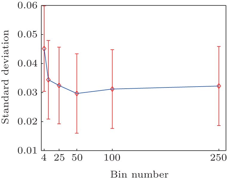 | Fig. B. Standard deviation of reconstructed distribution as a function of cell number. |
| 1 |
|
| 2 |
|
| 3 |
|
| 4 |
|
| 5 |
|
| 6 |
|
| 7 |
|
| 8 |
|
| 9 |
|
| 10 |
|
| 11 |
|
| 12 |
|
| 13 |
|
| 14 |
|
| 15 |
|
| 16 |
|
| 17 |
|
| 18 |
|
| 19 |
|
| 20 |
|
| 21 |
|
| 22 |
|
| 23 |
|
| 24 |
|
| 25 |
|
| 26 |
|
| 27 |
|
| 28 |
|
| 29 |
|
| 30 |
|
| 31 |
|
| 32 |
|
| 33 |
|
| 34 |
|
| 35 |
|
| 36 |
|
| 37 |
|
| 38 |
|
| 39 |
|
| 40 |
|
| 41 |
|
| 42 |
|