


Role of the aperture in Z-scan experiments: A parametric study
[Rashidian Vaziri M. R. ]
]
]
|
|


†Corresponding author. E-mail: rezaeerv@gmail.com
In close-aperture Z-scan experiments, a small aperture is conventionally located in the far-field thereby enabling the detection of slight changes in the laser beam profile due to the Kerr-lensing effect. In this work, by numerically solving the Fresnel–Kirchhoff diffraction integrals, the amount of transmitted power through apertures has been evaluated and a parametric study on the role of the various parameters that can influence this transmitted power has been done. In order to perform a comprehensive analysis, we have used a nonlinear phase shift optimized for nonlocal nonlinear media in our calculations. Our results show that apertures will result in the formation of symmetrical fluctuations on the wings of Z-scan transmittance curves. It is further shown that the appearance of these fluctuations can be ascribed to the natural diffraction of the Gaussian beam as it propagates up to the aperture plane. Our calculations reveal that the nonlocal parameter variations can shift the position of fluctuations along the optical axis, whereas their magnitude depends on the largeness of the induced nonlinear phase shift. It is concluded that since the mentioned fluctuations are produced by the natural diffraction of the Gaussian beam itself, one must take care not to mistakenly interpret them as noise and should not expect to eliminate them from experimental Z-scan transmittance curves by using apertures with different sizes.
For measuring refractive nonlinearities by the conventional Z-scan technique, a small aperture (or a pinhole) is normally used that ensures the measurement of only the on-axis transmission. In order to interpret the Z-scan experimental results, a simple analytic formula of the on-axis transmission was given in Ref. [1] under the Gaussian decomposition (GD) method proposed by Weaire et al., [2] in which they decomposed the complex electric field on the exit plane of the sample into a summation of Gaussian beams and then, simply considered the propagation of these Gaussian beams up to the aperture plane where they will be resumed to reconstruct the beam. Under the same approximation, the Z-scan theory has been further developed for media with nonlocal nonlinear response and a generalized analytic formula has been proposed for the on-axis transmission.[3, 4] However, both formulas are applicable when the size of aperture in the far-field is very small (pinhole) and the nonlinear phase shifts are not too large. It is obvious that the Z-scan theory based on the GD method is of limited practical use in most practical measurements since the aperture size and the nonlinear phase shifts are not always small. Hence, some theoretical treatments of the Gaussian beam Z-scan technique were developed, such as the aberration-free approximation[5] and the Fresnel– Kirchhoff theory, [6] to treat the cases with an arbitrary nonlinear phase shift or larger apertures.
Despite the aperture playing an important role in Z-scan experiments, no comprehensive study of its role has been done so far. Most of the studies done were based on the deriving approximate[7] and empirical[1] relations for the peak-to-valley transmittance differences on close aperture Z-scan curves. These relations contain a factor of (1 − S)n where 
In this work, instead of using approximate solutions for the far-field transmittance, we used the Fresnel– Kirchhoff diffraction integrals to more precisely study the role of the aperture in Z-scan experiments. In order to perform a comprehensive analysis, we used the nonlinear phase shift optimized for nonlocal nonlinear media.[3] In this way, it is also possible to study the role of nonlocality in Z-scan experiments using the Fresnel– Kirchhoff theory.
In Z-scan experiments, assuming that the sample has a cubic nonlinearity, then its intensity-dependent refractive index can be written as
 |
where n0 is the linear refractive index, n2 is the nonlinear refraction coefficient, and I denotes the laser beam intensity within the sample. Consider a fundamental Gaussian beam with a beam waist radius w0 traveling in the z direction, the complex electric field amplitude can be written as[4, 8]
 |
where 


At some distance z from the waist, the beam impinges on the surface of a nonlinear sample of width L. In the geometric-optics approximation, the sole effect of the nonlinear refractive index is to produce a phase shift, which varies across the beam profile.[2, 9] For a thin enough sample (L≪ z0) and by considering the possibility of the sample nonlocal response, [3, 10] this phase shift can be written as
 |
with
 |
where Δ Φ 0 is the maximum on-axis phase shift at the focus. The phenomenological parameter m is the order of nonlocality and can be any real positive number. For m < 1, the nonlinear phase change extends beyond the incident intensity distribution and for m > 1, the nonlinear phase change is narrower than the intensity distribution. Only for m = 1, the nonlinear phase change follows the intensity distribution and the sample response can be considered as local.
Now, the complex electric field exiting the sample Ee contains the nonlinear phase shift[11]
 |
In order to obtain the field distribution on the aperture plane, two procedures can be followed. First, using the GD method, [2] one can decompose the electric field in Eq. (5) into a summation of Gaussian beams and then resum them on the aperture plane after free propagation.[4] Second, the far-field intensity pattern on the aperture plane can be obtained by the free-space Fresnel– Kirchhoff diffraction integral at the Fraunhofer approximation[12, 13]
 |
where J0(k0θ r) is the first-kind zero-order Bessel function, θ is the far-field diffraction angle, ρ is the radial coordinate on the aperture plane at distance D, which is related to θ as ρ = (D − z)θ in the paraxial approximation, I0 is a constant, [14] and the total phase shift φ (z, r) is defined as
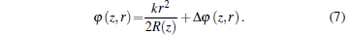 |
The first procedure has the advantage that it can yield a simple analytical formula for the on-axis transmission through the aperture for small nonlinear phase changes (| Δ Φ 0| ≪ π ).[4] This is made possible by retaining just the first two Gaussian components in the GD series.[4] Hence, this procedure is preferable for quickly evaluating the close-aperture Z-scan experimental results when the aperture size and the nonlinear phase change are both small enough. However, when one of these conditions is not satisfied, the mentioned analytical formula of the on-axis transmission for determining the nonlinear index of refraction of materials cannot be used. For instance, for large nonlinear phase shifts, one can retain higher Gaussian beam components in the GD series which do not lead to simple analytical formulas.[15] Furthermore, retaining some higher-order components is not a precise enough method since inevitably one must give up many more components in the GD series. In these conditions, one can use the second procedure to precisely consider the role of larger apertures and nonlinear phase shifts in Z-scan experiments.
Using Eq. (6), the normalized transmittance (NT) through the aperture can be calculated as
 |
where a is the aperture radius. Therefore, the normalized transmittance through the far-field aperture can be calculated by numerically solving the integrals in Eq. (8). In this way, it is possible to make a parametric study of the role of various parameters, like a, Δ Φ 0, and m, in Z-scan experiments. For numerical evaluation of the normalized transmittance, the constants n0, λ , and D were chosen as 1, 532 nm, and 2.28 m, respectively.
Initially, in order to test the accuracy of our numerical method, we have calculated the NTs by setting ρ equal to zero in Eq. (8), i.e., we have calculated the on-axis NTs. Figure 1 shows the NT curves for different values of the nonlocal parameter m. Different symbols indicate the curves that have been depicted using the on-axis NTs from the generalized nonlocal Z-scan theory[3]
 |
The excellent correspondence between the two sets of curves confirms the accuracy of our numerical analysis.
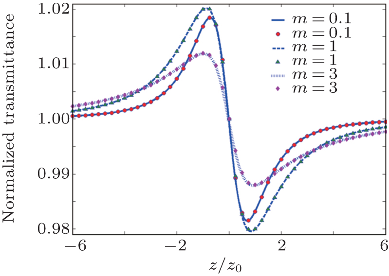 | Fig. 1. Two sets of NT curves corresponding to numerical evaluation of Eq. (8) and applying the analytical formula in Eq. (9) (symbols). Values of the nonlocal parameter m have been chosen so as to consider the three different possibilities: the local case (m = 1), the wider (m < 1), and the narrower ( m > 1) distributions of the nonlinear phase shift compared to the field intensity distribution. [3, 10] The Δ Φ 0 has been set to 0.1 to ensure the smallness of the nonlinear phase shift required by the Z-scan theory based on the GD analysis.[1, 3] |
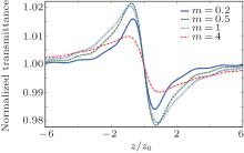
In Fig. 2, NT curves have been depicted for an aperture radius equal to 0.1 mm and for different values of m. The NT curves in Fig. 2 are quite similar to the curves in Fig. 1 aside from the important fact that by moving away from the focal point (z = 0), some fluctuations become visible on the curves. These fluctuations are observable symmetrically in both sides of the focal point and since in the on-axis case in Fig. 1 no trace of them can be found, their appearance can be attributed to the use of an aperture with a finite radius. These types of symmetrical fluctuations can be seen on experimental NT curves of the seminal work of Sheik-Bahae et al.[1] and also on experimental NT curves of other later reports.[16– 21] However, to the best of our knowledge, despite their widespread occurrence, no systematic work has been done so far to explain the reason why these symmetrical fluctuations appear on Z-scan NT curves.
 | Fig. 2. Z-scan NT curves with different values of m when a small aperture with radius of 0.1 mm is used in simulations. The on-axis phase shift Δ Φ 0 has been set equal to 0.1. |
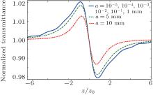
Figure 3 shows the Z-scan NT curves for different values of aperture radius. Inspecting this figure, it is clear that the apertures that are typically used in Z-scan experiments will inevitably result in the formation of fluctuations on the wings of NT curves. It is also obvious that the aperture size has negligible effect on the shape and position of these fluctuations. By increasing the aperture radius further than 1 mm, gradually smoother NT curves will be formed. Indeed, for apertures with radius greater than 5 mm, one would gradually meet the open-aperture Z-scan experimental conditions and hence the intensity of the extrema will decrease. When the aperture is completely removed, or mathematically for infinitely large values of the aperture radius, the NT curves will change into straight lines which lie on the horizontal axis.
 | Fig. 3. A closer look at the role of aperture size in Z-scan experiments. For obtaining the NT curves, values of Δ Φ 0 and m have been set equal to 0.1 and 1, respectively. |
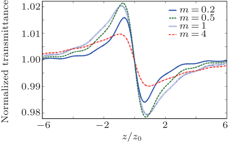
In Fig. 4, the role of Δ Φ 0 variations on Z-scan NT curves has been investigated. A noticeable asymmetry around the origin has been developed on the NT curves for large values of the nonlinear phase shift. This asymmetry, which is not present on the NT curves of Figs. 1– 3, becomes more pronounced for larger values of the nonlinear phase shift. For Δ Φ 0 values equal to or greater than 2π , the NT reaches a value equal to zero near the origin; a fine structure develops around the valleys and intensity of the peaks greatly increases. All of these features, have been previously reported to be formed on the on-axis NT curves.[6, 15, 22] Aside from all the mentioned features, one must also notice that the symmetrical fluctuations due to the presence of aperture become more pronounced for larger values of the nonlinear phase shift.
 | Fig. 4. Role of the nonlinear phase shift variations on Z-scan NT curves. During the computations, values of the nonlocal parameter m and the aperture radius a have been set equal to 0.5 and 0.1 mm, respectively. |
From Figs. 2– 4, one can conclude that the nonlocal parameter variations can shift the position of fluctuations, which appear on NT curves when an aperture is used in Z-scan experiments, along the optical axis, whereas their magnitude depends on the largeness of the induced nonlinear phase shift.
Now, we are at the position to discuss the possible reason for the formation of symmetrical fluctuations on the wings of close-aperture Z-scan NT curves. It is well known that when an intense laser beam passes through a nonlinear Kerr medium, its spatial profile changes as a consequence of laser-matter interaction and after exiting the medium, a set of concentric rings can be observed on a far-field screen.[12, 23, 24] In Z-scan experiments, the aperture should be placed at the far-field and hence one should always keep in mind the possibility of ring formation on its plane that can alter the amount of radiation which passes through it. Equation (6) represents the integral which is mostly used for interpreting these concentric rings.[13] In this equation, the total phase shift φ (z, r) determines the form of the obtainable rings. Equation (7) shows that the total phase shift contains two terms where the first term is related to the beam radius of curvature R(z) and the second term, according to Eqs. (3) and (4), is related to the nonlinear phase shift. When equation (7) is inserted into Eq. (6), its first term determines the natural beam diffraction and its second term determines the diffraction rings due to the nonlinear Kerr effect.[25] For small values of the nonlinear phase shift, like Δ Φ 0 = 0.1 which is used for depicting the NT curves in Figs. 2 and 3, the second term cannot contribute to the formation of rings at far-field. In fact, it is previously shown that just for Δ Φ 0 values much larger than 2π diffraction rings due to the nonlinear action of the medium can be formed at the far-field.[12, 13, 25] Therefore, the observed fluctuations in Figs. 2 and 3 can be produced by the change in the form of the natural diffraction rings, when the sample moves along the optical axis. In order to examine this possibility in more detail, in Fig. 5, we have shown the normalized intensity distributions on the aperture plane for different positions of the sample along the optical axis. For determining these normalized intensity distributions, m and Δ Φ 0 have respectively been chosen as unity and 0.1. The other constants have been the same as those used for obtaining the NT curves in Figs. 1– 4. As can be seen, the sample movement along the optical axis has the accompanying effect of changing the normalized intensity distribution, specifically near the radial coordinate origin (ρ = 0). By moving the sample further than 3z0 away from the focal point (z = 0), gradually the Gaussian shape of the intensity distribution becomes distorted and these distortions lie in the range which is normally covered by conventionally used apertures in Z-scan experiments. This supports our previous idea that the observed fluctuations on Z-scan NT curves must be due to the natural diffraction of the Gaussian beam itself after exiting from the sample.
 | Fig. 5. The normalized beam intensity distributions versus the radial coordinate on the aperture plane. Distributions have been obtained on the aperture plane when the sample is located at different positive multiples of the Rayleigh length along the optical axis in Z-scan experiments. |
To detect the lensing effect of the nonlinear samples, conventionally, a finite size aperture is used in close-aperture Z-scan experiments. In this way, for samples with positive and negative refractive nonlinearities, valley-to-peak and peak-to-valley shapes will be obtained in Z-scan NT curves, respectively.[1] For evaluating the NT curves and measuring the nonlinear index of refraction, an analytical approach based on the GD method has been proposed because its simplicity is widely used.[1, 3] However, the established relations in this method are for the on-axis transmission and when a finite size aperture is used in Z-scan experiments, one should resort to more precise methods. In this paper, the amount of transmission through finite size apertures has been calculated using the Fresnel– Kirchhoff diffraction integrals. Our calculation results show that apertures will result in the formation of symmetrical fluctuations on the wings of Z-scan NT curves. These kinds of fluctuations cannot be described by the analytical relations, like Eq. (9), of the aforementioned simplified approach based on the GD method. It is shown that the appearance of these fluctuations on Z-scan NT curves can be ascribed to the natural diffraction of the Gaussian beam, as it propagates up to the aperture plane. Our simulation results indicate that the natural beam diffraction will cause the formation of slight distortions in the Gaussian beam intensity profile on the aperture plane which are mostly concentrated around the aperture center. Therefore, the conventionally used apertures in Z-scan experiments, with radii around tens or hundreds of micrometers, can detect these slight distortions during the sample movement along the optical axis whose overall effect appears as the observed fluctuations on NT curves.
Since the observed fluctuations on Z-scan NT curves are shown to be due to the natural beam diffraction, one must take care not to mistakenly interpret them as noise. Indeed, these fluctuations have been produced by the signal itself. Therefore, it should not be expected that by changing the aperture size, these fluctuations could be eliminated from the close-aperture Z-scan NT curves.
| 1 |
|
| 2 |
|
| 3 |
|
| 4 |
|
| 5 |
|
| 6 |
|
| 7 |
|
| 8 |
|
| 9 |
|
| 10 |
|
| 11 |
|
| 12 |
|
| 13 |
|
| 14 |
|
| 15 |
|
| 16 |
|
| 17 |
|
| 18 |
|
| 19 |
|
| 20 |
|
| 21 |
|
| 22 |
|
| 23 |
|
| 24 |
|
| 25 |
|