


Stark-potential evaporative cooling of polar molecules in a novel optical-access opened electrostatic trap
[Sun Hui, Wang Zhen-Xia, Wang Qin, Li Xing-Jia, Liu Jian-Ping, Yin Jian-Ping ]
]
]
|
|


†Corresponding author. E-mail: jpyin@phy.ecnu.edu.cn
We propose a novel optical-access opened electrostatic trap to study the Stark-potential evaporative cooling of polar molecules by using two charged disk electrodes with a central hole of radius r0 =1.5 mm, and derive a set of new analytical equations to calculate the spatial distributions of the electrostatic field in the above charged-disk layout. Afterwards, we calculate the electric-field distributions of our electrostatic trap and the Stark potential for cold ND3 molecules, and analyze the dependences of both the electric field and the Stark potential on the geometric parameters of our charged-disk scheme, and find an optimal condition to form a desirable trap with the same trap depth in the x, y, and z directions. Also, we propose a desirable scheme to realize an efficient loading of cold polar molecules in the weak-field-seeking states, and investigate the dependences of the loading efficiency on both the initial forward velocity of the incident molecular beam and the loading time by Monte Carlo simulations. Our study shows that the maximal loading efficiency of our trap scheme can reach about 95%, and the corresponding temperature of the trapped cold molecules is about 28.8 mK. Finally, we study the Stark-potential evaporative cooling for cold polar molecules in our trap by the Monte Carlo method, and find that our simulated evaporative cooling results are consistent with our developed analytical model based on trapping-potential evaporative cooling.
Over the past few years, the interest in trapping and cooling cold polar molecules is rapidly growing. In 2000, Meijer’ s group proposed the first trap scheme for ND3 molecules in the electrostatic field of the weak-field-seeking (WFS) states.[1] Then, they achieved an ac electric trap for ground-state molecules, which was capable of confining neutral atoms and molecules in both weak-field-seeking and high-field-seeking states; [2] and trapping of 15ND3 ammonia molecules in a cylindrically symmetric ac trap was demonstrated[3] later. In 2007, Ye’ s group reported a scheme of magnetoelectrostatic trapping of ground-state OH molecules at a density of ∼ 3 × 103 cm− 3 and temperature of 30 mK.[4] In the same year, Kleinert et al. described the realization of a dc electric field trap for ultracold polar molecules with the thin wire electrostatic trap, [5] and the cold molecules in the WFS states could be trapped in a half-opened linear ac trap.[6] In 2008, molecular beam collision with a magnetically trapped target was realized experimentally by Ye’ s group.[7] In 2012, Ye’ s group studied the evaporative cooling of the dipolar hydroxyl radical OH and showed the relationship of the final observed temperature versus the effective trap depth and the final temperature and calculated the relative phase-space density versus the remaining relative molecule number.[8] In the next year, Holland described the evaporative cooling of reactive polar molecules KRb confined in a two-dimensional geometry and that a considerable increase in phase-space density could be achieved via evaporative cooling.[9] Our group has also made some progress in this field. In 2013, we proposed an optically accessible electrostatic trap scheme to confine cold polar molecules by using two charged spherical electrodes, but the maximal loading efficiency could reach only ∼ 14%, [10] followed by an electrostatic trap for cold polar molecules on a chip with a loading efficiency of about 11.5%.[11] Recently, we proposed a novel electrostatic trap scheme with a high loading efficiency of ∼ 67%.[12]
In this paper, we demonstrate a simpler scheme to realize a highly efficient electrostatic trap for cold polar molecules by using an optical-access opened electrostatic field generated by two charged disks, theoretically prove its feasibility by Monte Carlo simulations, and then study the evaporative cooling of polar molecules in our scheme. In Section 2, we derive a set of analytical solutions to calculate the electric field distributions and Stark potential for ND3 molecules and analyze the dependences of the efficient trapping potential on the geometric parameters of our trap scheme. In Section 3, we study the loading and trapping processes of cold ND3 molecules by Monte Carlo simulations, and analyze the dependences of the loading efficiency on both the loading time and the initial velocity of the incident cold molecular beam. In Section 4, we study the Stark-potential evaporative cooling of cold polar molecules. We use a simple analytic model and compare the analytical results with the simulated ones obtained by the Monte Carlo method. In the final section, we summarize the main results and conclusions.
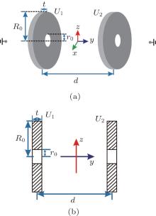
Figure 1(a) shows the 3D layout of our electrostatic trap scheme with two charged disk electrodes of radius R0, and a hole of radius r0 is drilled on both of them. The thickness of the two disks is t, and the distance between their centers is d. Assuming that the potential at infinity is 0, we apply high voltages U1 and U2 to the left and the right disks, respectively. Figure 1(b) shows the projection of the double-disk layout in the yz plane.
 | Fig. 1. (a) Schematic diagram of electrostatic trap with two charged disk electrodes. The radius of the disk is R0, the radius of the hole is r0, the thickness of the two disks is t, and the distance between the centers of them is d. The potential at infinity is 0 and the voltages applied to the two disks are U1 and U2, respectively. (b) Projection of double-disk layout in the yz plane. |
We derive a set of analytical solutions to analyze the electrostatic field distributions generated by the two charged disk electrodes, which are applied with a high voltage U. At first, we calculate the electrostatic potential of our trap scheme in the spherical coordinate system, and then by transformation of the coordinate systems, we can obtain the analytical solution of the electrostatic potential in the Cartesian coordinate system, which is approximately given by[13]
 |
where σ is the density of surface charge, ɛ 0 is the permittivity of a vacuum, and b is a parameter related to the distance between the centers of the two disks and the thicknesses of the two disks, i.e., b = d/2− t/2. According to the Poisson equation, [11] we can calculate the electric field distribution of our trap scheme in the y direction by
 |
From Eq. (2), we calculate the integral of Ey from d/2 + t/2 to ∞ to obtain the relationship between the voltage U and the density of surface charge σ ,
 |
where A′ (x, y, z) is a parameter that we introduced. Assuming
 |
when R0 = 10 mm, r0 = 1.5 mm, d = 20 mm, t = 2 mm, and U = 10 kV, we have A ≈ 10.278 mm. So the relationship between the voltage U and the density of surface charge σ can be expressed as
 |
According to Eqs. (1) and (5), we can obtain the analytical solutions to calculate the electric field distribution of the trap layout. The relationship between the generated electrostatic field and the geometric parameters is given as follows:
 |
 |
 |
 |
Then we calculate the corresponding Stark trapping potential by the following equation:[3]
 |
where Winv is the inversion splitting, μ is the electric dipole moment of the trapped molecules, J is the rotational quantum number of a molecular electric state, and K and M are the projections of the total angular momentum on the molecular axis and the space fixed axis, respectively. Here we assume that the cold ND3 molecules come from a Stark decelerated molecular beam in a single WFS state of | J, K, M 〉 = | 1, 1, − 1〉 . Then the molecules in WFS can be repelled to the minimum of the electrostatic field by the repulsive gradient force, which is given by
 |
By using Eq. (11) and according to the Newtonian motional equation F = ma, we can study the dynamical processes of the loading, trapping, and cooling of cold polar molecules in our proposed electrostatic trap by means of Monte– Carlo simulations.
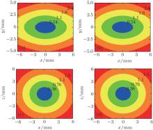
We calculate the contour distributions of the electric field in the xy and xz (yz) planes for R0 = 10 mm, r0 = 1.5 mm, t = 2 mm, d = 20 mm, and U = 10 kV, as shown in Figs. 2(a) and 2(c). To verify the accuracy of our analytical solutions, we calculate the contour distributions by a commercial finite-element software (Maxwell) and the results are shown in Figs. 2(b) and 2(d). We find that our analytical results are nearly consistent with the numerical ones, which proves that the above derived equations can be used to calculate the E-field distribution of our trap scheme. What is more, the field distribution is 3D closed and the lowest field strength is at the origin which can be used to confine the cold molecules in WFS states.
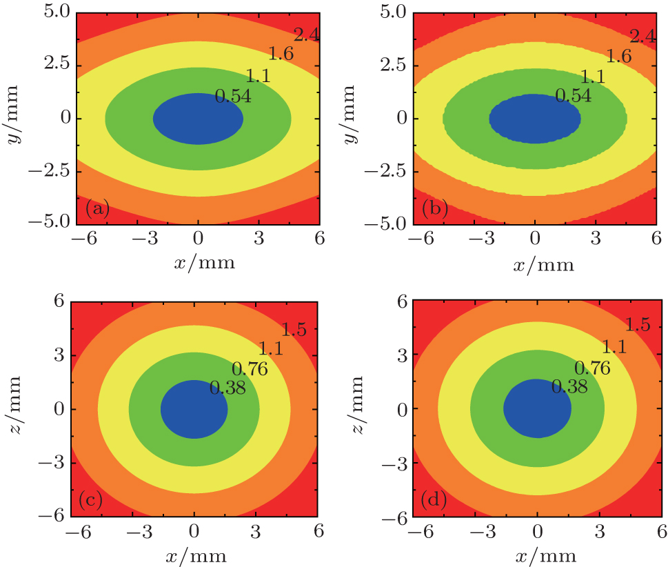 | Fig. 2. (a), (c) The calculated contour distributions from our analytical solutions and (b), (d) the numerically calculated contour distributions from a commercial software (Maxwell) in the xy (zy) and xz planes for R0 = 10 mm, r0 = 1.5 mm, t = 2 mm, d = 20 mm, and U = 10 kV. The labels are all in units of kV/cm. |
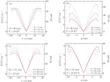
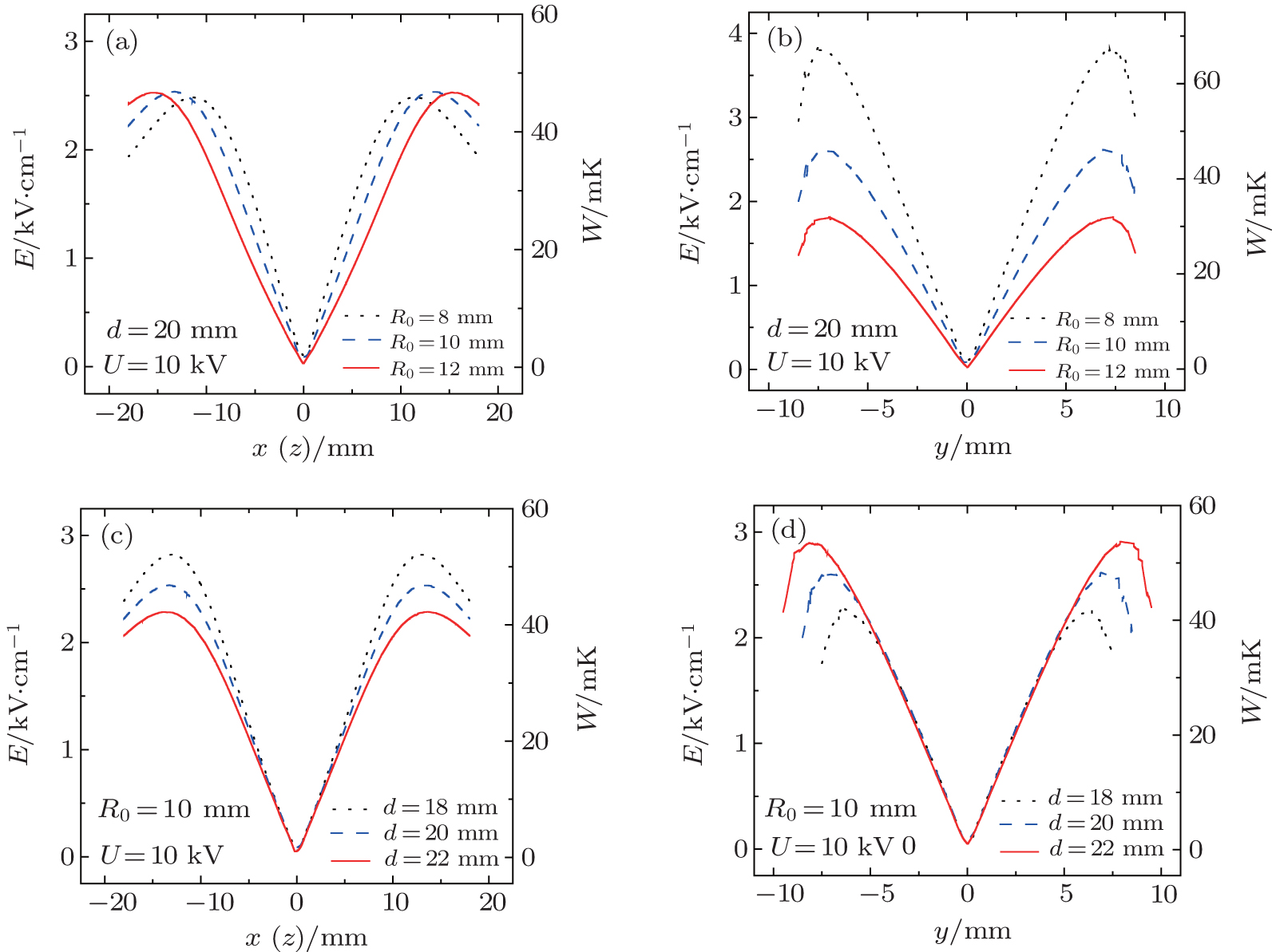 | Fig. 3. Spatial distributions of the electrostatic field and the Stark trapping potential for ND3 molecules in the x, y, and z directions for different disk radius R0 when d = 20 mm, r0 = 1.5 mm, t = 2 mm, and U = 10 kV, and for the difference distance d between the two disk centers when R0 = 10 mm, r0 = 1.5 mm, t = 2 mm, and U = 10 kV. Here panels (a) and (c) are the results in the x (z) direction, and panels (b) and (d) are ones in the y direction. |
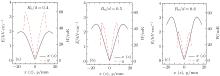
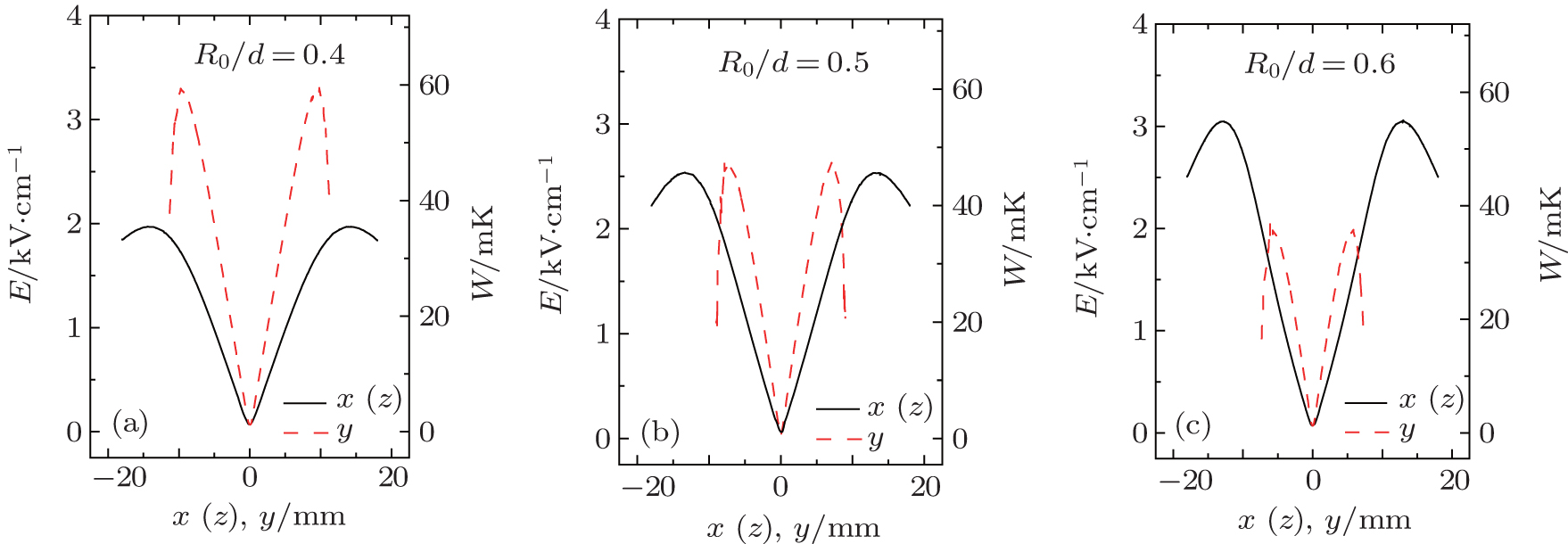 | Fig. 4. Relationship between the effective trap depth and the ratio R0/d: (a) R0/d = 0.4, (b) R0/d = 0.5, (c) R0/d = 0.6; where R0 = 10 mm, and d = 25 mm, 20 mm, and 16.6 mm, respectively. The solid black curve represents the effective trap depth in the x or z direction, and the dashed red curve represents the effective trap depth in the y direction. |
Then we study the dependences of the electric field on the radius R0 and the distance d between the two disk centers, and the results are shown in Fig. 3. From Figs. 3(a) and 3(b), we can see that with the increase of the radius R0, the maximum electric field strength in the x and z directions will increase slowly, while that in the y direction will have an apparent decline. According to Figs. 3(c) and 3(d), we can find that with the increase of the distance d, the effective well depth in the x and z directions will be decreased, while that in the y axis will be increased. From these dependences, we find that the trap will become deeper if the distance between the two disk electrodes decreases or the radius of the disk electrode increases. Then we study the dependence of the effective well depth on the ratio of the radius of the disks R0 to the spacing between the two disks d, and the results are shown in Fig. 4. We find that when R0/d = 0.5, the effective well depths in the x, y, and z directions are nearly the same, while for R0/d = 0.4 and 0.6, the effective well depths differ largely between the x (z) direction and the y direction. In particular, when R0 = 10 mm and d = 20 mm, the effective trap depths in the x, y, and z directions are all about 50 mK, which is deep enough to trap cold ND3 molecules of about 20 mK produced in our lab. In order to obtain a high loading and trapping efficiency in the following discussion, we will apply larger voltages of 30 kV and 50 kV to the electrodes.
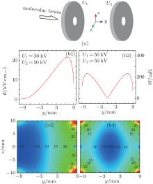
As shown in Figs. 5(a) and 5(b1), we apply a voltage U1 = 30 kV to the left disk and U2 = 50 kV to the right disk to realize an efficient loading for ND3 molecules; here R0 = 10 mm, r0 = 1.5 mm, d = 20 mm, and t = 2 mm. We calculate the field distributions in the y direction and the corresponding contour distributions in the yz plane. The results are shown in the left parts of Figs. 5(b1) and 5(b3). With the increase of the electrostatic field in the y direction, the WFS ND3 molecules will feel a repulsive force and then slow down. Then we increase the voltage of U1 to 50 kV on the condition that the other parameters are unchanged to form an efficient trapping, the results are shown in the right parts of Figs. 5(b2) and 5(b4). The incident ND3 molecules that are decelerated to nearly 0 can be trapped in the center of our layout.
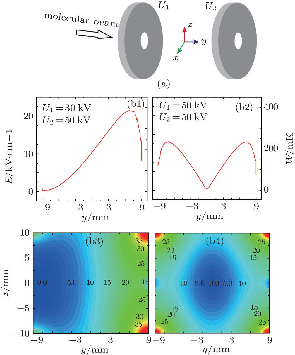 | Fig. 5. (a) Schematic diagram of the two charged disks used for efficient loading of cold molecules. (b) The electric field profiles in the y direction and the contour distributions in the yz plane for the loading (left column, when U1 = 30 kV, U2 = 50 kV) and trapping (right column, when U1 = U2 = 50 kV) of cold polar molecules. |
We perform Monte Carlo simulations to calculate the dynamical loading and trapping efficiency of cold ND3 molecules. The simulated molecular number is 105 and the initial spatial distributions and velocity profiles of the incident pulsed ND3 molecular beam are both Gaussian ones. We assume that the diameter of the incident ND3 molecules is 3 mm, the initial transverse velocity of the molecules is zero, and the full widths at half maximum (FWHM) of the velocity distributions in the x, y, and z directions are all 3 m/s. Then we select a molecule and study its motion in our loading and trapping process. According to Newton’ s second law, we can obtain the position and velocity of the selected molecule at any moment. When it moves to the central region of the trap, we can obtain the loading time tload, which can then be used to load all the incident cold molecules. Once t = tload, we switch the loading electric field to the trapping one. In the end, we can obtain the position and velocity of every stable molecule trapped in the central region, which can be used to calculate the spatial and velocity distributions of the cold molecules. The simulated results are shown in Figs. 6 and 7.
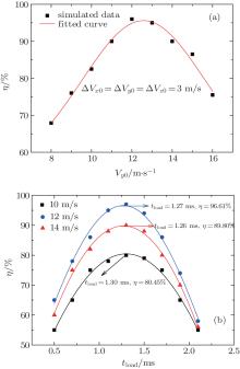
Figure 6(a) shows the dependence of the loading efficiency of the cold molecules on the central velocity Vy0 of the incident molecular beam. When Vy0 = 12 m/s, we can achieve the highest loading efficiency of cold molecules about 95%. Figure 6(b) shows the dependence of the loading efficiency on the loading time for different initial central velocities of the cold molecular beams. There is a corresponding optimal loading time when the velocity is Vy0 = 10 m/s, 12 m/s, and 14 m/s. In particular, when Vy0 = 12 m/s, we can obtain the optimal loading time of about 1.27 ms, which we can use to realize the best loading efficiency.
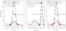
Figure 7 shows the initial and the final velocity distributions of the cold ND3 molecules in the loading and trapping processes. We can see that the central velocities in the x and z directions are nearly the same due to the symmetry, while the velocity in the y direction is decelerated from 12 m/s to about 0. What is more, the FWHM of the final velocity distributions in the x, y, and z directions are about 5.38 m/s, 9.26 m/s, and 5.56 m/s, respectively. Then we can find that the 3D temperature of the trapped cold molecules is about 28.8 mK.
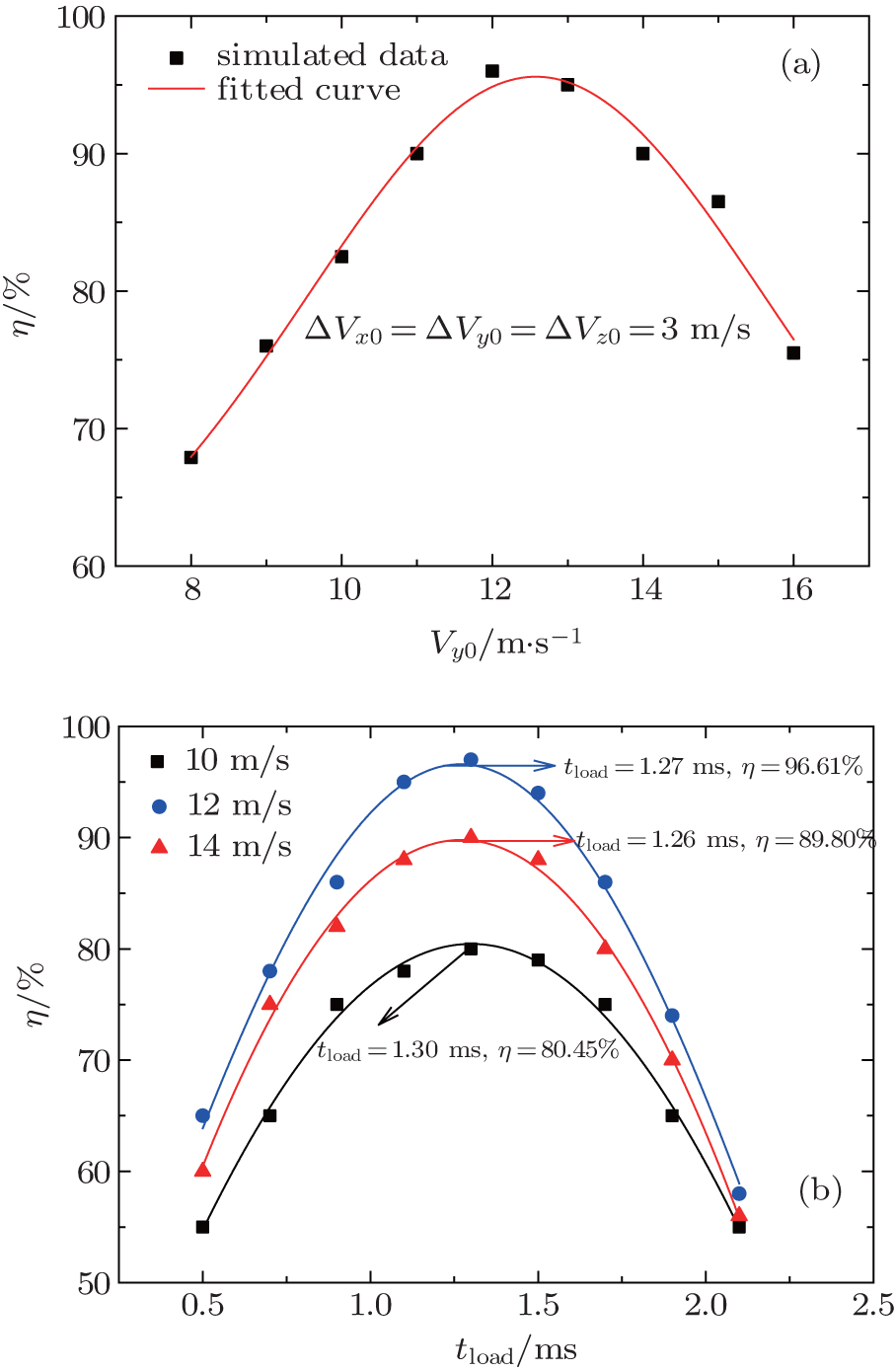 | Fig. 6. Dependences of the loading efficiency of cold ND3 molecules on (a) the initial central velocity Vy0 of the incident ND3 molecular beam for Δ Vx0 = Δ Vy0 = Δ Vz0 = 3 m/s and (b) the loading time tload for different initial central velocities (Vy0 = 10 m/s, 12 m/s, 14 m/s). The data points are the simulated results, and the solid lines are the fitted curves. |
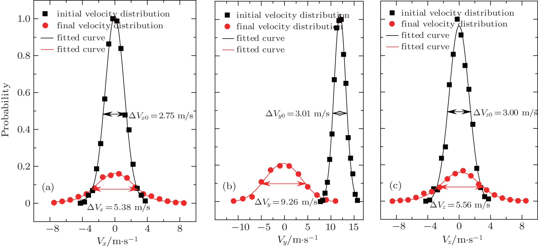 | Fig. 7. Initial (black) and final (red) velocity distributions of cold ND3 molecules in the (a) x, (b) y, and (c) z directions during the loading and trapping processes of the cold ND3 molecules in the double-disk trap. The data points are the simulated results, and the solid lines are the fitted curves. |
In 1995, Ketterle’ s group proposed a simple analytical model to describe the temperature change of the trapped molecules during the trapping-potential evaporative cooling process, and gave five hypotheses, including pure S-wave scattering and completely evaporative cooling, etc. Here we only briefly introduce the basic main points of this simple analytical model of evaporative cooling, [14] including only elastic collisions, evaporative loss of particles, and background gas collisions. First of all, assuming that ɛ i (i = 1, 2, 3) is the unit energy in three dimensions, ai (i = 1, 2, 3) is the characteristic length of the potential well in three dimensions, and Si (i = 1, 2, 3) is the power exponent of the potential energy in three dimensions, we can give the potential energy of the trapping well in the Cartesian coordinate system as[14]
 |
Introduce a parameter to describe the characteristics of the potential well and define it as
 |
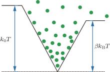
For a given temperature, the parameter ξ has an important impact on the trapping volume. In view of a 3D linear potential well, we can take S1 = S2 = S3 = 1, so ξ = 3. For simplicity, we firstly study one step of evaporative cooling. As shown in Fig. 8, we assume that the initial number of molecules in the trap is N0 and the initial temperature of molecules is T0. After one step of evaporative cooling, the trap depth is decreased from kBT to β kBT. We define two parameters:[12]
 |
 |
where N is the number of molecules still remaining in the trap after one step of evaporative cooling, and T is the corresponding temperature. According to Eqs. (14) and (15), we obtain
 |
Considering that the trapping volume satisfies V ∝ Tξ , we can obtain
 |
where V0 is the initial trapping volume of molecules. According to Eqs. (14) and (17), we can obtain the number density of the trapped molecules as follows:
 |
where n0 is the initial density of the trapped molecules. Because the phase-space density of the trapped molecules satisfies 
 |
where ρ 0 is the initial phase-space density of the trapped molecules.
If the process of the above evaporative cooling can be repeated by a number of j steps, we only replace v with vj to obtain the changes of the related physical quantities.[14]
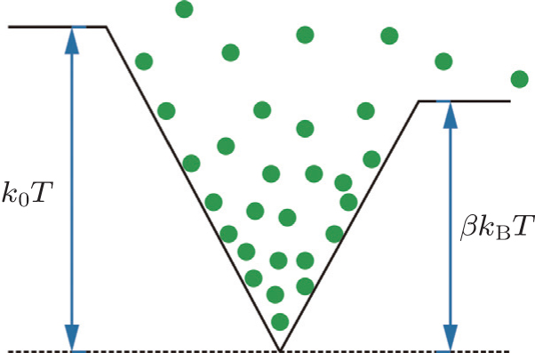 | Fig. 8. A simple analytic model for evaporative cooling of cold molecules in a three-dimensional linear potential well. The kBT is the initial trap depth, and β kBT is the trap depth after one step of evaporative cooling. |
It is well known that if the depth of an efficient potential well is lowered, the temperature, volume, number, and number density of the trapped molecules will be reduced, and the corresponding phase-space density will be increased due to evaporative cooling. Here we use our electrostatic trap scheme to study the evaporative cooling for ND3 molecules by lowering the depth of our potential well.
At first, we apply a voltage of 50 kV to generate an initial trapping depth, then we decrease the voltage by 5 kV every 100 ms until the voltage is reduced to 5 kV. To verify if the trapped molecules get a net evaporative cooling, we study the change of the molecular temperature with the decrease of the voltage applied to the two disks from 50 kV to 5 kV, and the simulated results are shown in Fig. 9. From Eq. (17), we can obtain the temperature of the trapped molecules after the evaporative cooling as follows:
 |
where U0 is the initial voltage applied to the two charged disks. In Fig. 9, the data points are the simulated results, and the solid red lines are the calculated results from Eq. (20), that is, an analytical model of the evaporative cooling, while the dashed blue lines are the calculated ones from Eqs. (10) and (11), that is, an analytical model of the adiabatic cooling of cold molecules in a linear trap. We can see from Fig. 9 that our simulated results are consistent with the ones of the theoretical calculation only when the voltage is lower than about 10 kV for evaporative cooling. When the voltage is higher than 20 kV, the adiabatic cooling plays a major role, so we apply the voltage of 10 kV to generate an initial trapping depth, as a starting point, so as to study the evaporative cooling of the molecules in our trap. After the number of molecules in the trapping well is almost constant, we obtain the corresponding number and temperature of molecules, which are about N0 = 104 and T0 = 9.3 mK, respectively.
 | Fig. 9. The change of the ND3 molecular temperature with the decrease of the voltage applied to the two charged disks from 50 kV to 5 kV. (a) The change of the temperature in the x or z direction, (b) the change of the temperature in the y direction, and (c) the change of the 3D temperature. The data points are the simulated results, the solid red lines are the calculated curves from the analytical model of evaporative cooling, and the dashed blue lines are the simulated curves. |
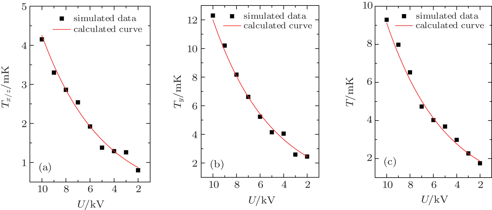 | Fig. 10. The change of the ND3 molecular temperature with the decrease of the voltage applied to the two charged disks from 10 kV to 2 kV. (a) The change of the temperature in the x or z direction, (b) the change of the temperature in the y direction, and (c) the change of the 3D temperature. The data points are the simulated results, and the solid red lines are the calculated curves from the analytical model of evaporative cooling. |
 | Fig. 11. The changes of (a) the number of trapped molecules, (b) the trapping volume, (c) the number density of trapped molecules, and (d) the phase-space density of trapped molecules with the decrease of the voltage applied to the two charged disks from 10 kV to 2 kV during evaporative cooling. The data points are the simulated results, and the solid red lines are the calculated curve from the analytical model of evaporative cooing. |
Then we lower the voltage by 1 kV every 100 ms until the voltage is reduced to 2 kV. Figure 10 shows the changes of the molecular temperature with the decrease of the voltage from 10 kV to 2 kV. Figure 10(a) shows the change of the temperature in the x or z direction, figure 10(b) is the change of the temperature in the y direction, and figure 10(c) shows the change of the 3D temperature. The data points are the simulated results, and the solid lines are the calculated ones from Eq. (20). We can see from Fig. 10 that with the lowering of the voltage from 10 kV to 2 kV, the translational temperature of the molecules in the x or z direction is decreased from 4.21 mK to 0.79 mK, the translational temperature of the molecules in the y direction is reduced from 12 mK to 2.34 mK, and the 3D translational temperature is decreased from 9.29 mK to 1.75 mK. In addition, our simulated results are in good agreement with the ones of the theoretical calculation from Eq. (20).
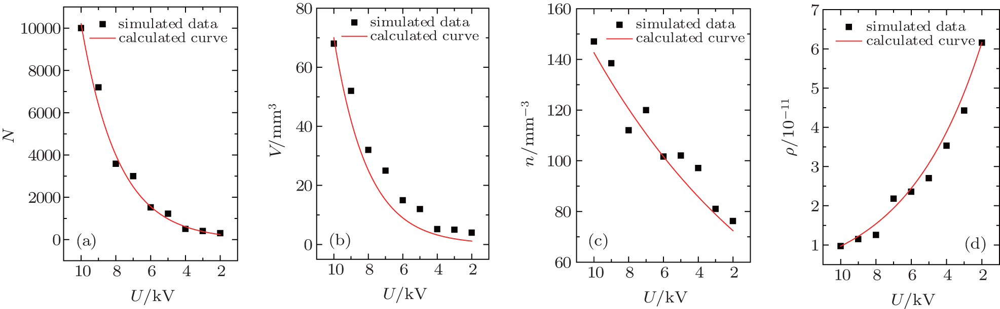
Then we study the change of the molecular number (N), the trapping volume (V), the density of trapped molecules (n), and its phase-space density (ρ ) with the lowering of the voltage from 10 kV to 2 kV; the results are shown in Fig. 11. The data points are the simulated results and the solid lines are fitted by the following equations:
 |
 |
 |
 |
where N0 is the initial number of molecules after being trapped with the voltage of 10 kV for 100 ms, V0 and n0 are the corresponding initial trapping volume and density of the trapped molecules, v is the residual ratio, U is the trapping voltage in units of kV, γ is a parameter used to describe the decrease of temperature due to the loss of hot molecules, and ξ is a parameter related to the dimensions and the shape of the potential well. We can see from Fig. 11 that with the decrease of the voltage from 10 kV to 2 kV, the number of molecules trapped in our electrostatic well will be decreased from 10000 to 305, the trapping volume is reduced from 68 mm3 to 3 mm3, and the density of the trapped molecules is decreased from 145 mm− 3 to 75 mm− 3. We can also find that our simulated results are well consistent with the ones of the theoretical calculation from Eqs. (21)– (24).
Finally, we show the contour distributions of the electrostatic field in the yz plane with the decrease of the voltage and study the corresponding spatial distributions of the trapped molecules during the evaporative cooling, and the results are shown in Fig. 12. The left column shows the contour distributions of the trapping field when the voltage applied to the two disks is 10 kV, 8 kV, 6 kV, 4 kV, and 2 kV, respectively. The right column shows the corresponding spatial distributions of the molecules in the yz plane. We can see from Fig. 12 that with the lowering of the voltage, the efficient well depth in the yz plane becomes shallower, and the volume, number of the trapped molecules, and its density will be greatly reduced, which are consistent with the simulated results shown in Figs. 11(a)– 11(c).
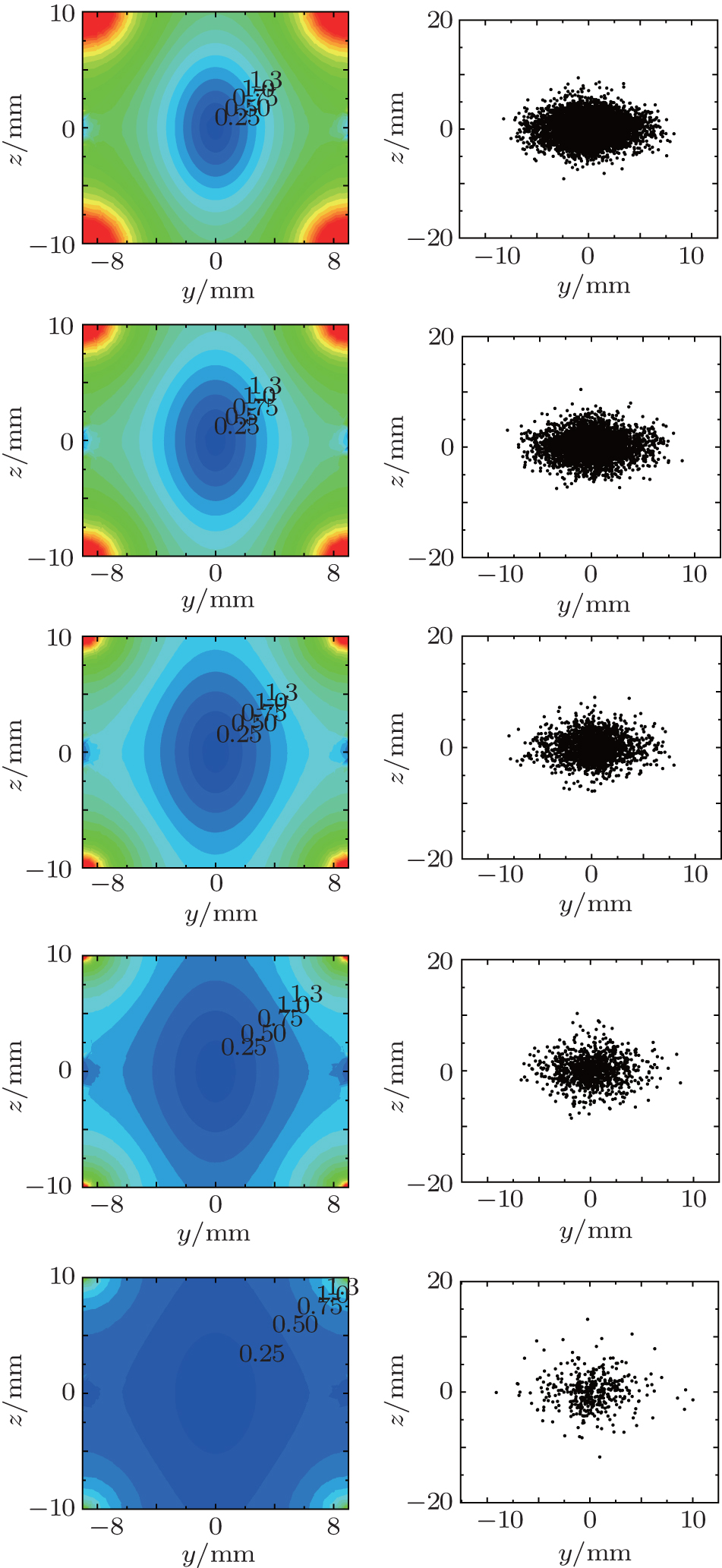 | Fig. 12. The left column shows the contour distributions of the electrostatic field in the yz plane when the voltage applied to the two disks is (a) 10 kV, (b) 8 kV, (c) 6 kV, (d) 4 kV, and (e) 2 kV, respectively. When the molecules are stable in our electrostatic trap, we decrease the voltage by 2 kV every 50 ms. The right column shows the corresponding spatial distributions of the trapped molecules in the yz plane. |
In this paper, we have proposed an optical-access opened electrostatic trap scheme to study the evaporative cooling of polar molecules by using two charged disk electrodes with a central hole. Then we have studied the dependences of the electrostatic field and its Stark trapping potential for ND3 molecules on the radius of the disk electrode and the distance between the centers of the two charged disks. What is more, we have proposed a desirable scheme to load and trap cold polar molecules by changing the voltage on the left disk from 30 kV to 50 kV. Our study shows that when Vy0 = 12 m/s, tload = 1.27 ms, the loading efficiency can reach its maximum ∼ 95% and the corresponding temperature is ∼ 28.8 mK. In addition, we have studied the Stark-potential evaporative cooling in our electrostatic scheme for cold polar molecules and found that theoretically calculated results of Ketterle’ s analytical model for evaporative cooling are well consistent with our simulated results.
Some unique advantages, such as the simplest electrode structure, completely opened optical access, and the highest loading efficiency, are the most important features of our trap scheme. In addition, our proposed electrostatic trap has some physical applications such as cold collisions, [15, 16] cold chemistry, [17] high-resolution spectroscopy, [18, 19] the ealization of molecular Bose– Einstein condensate, [20] and laser cooling of neutral molecules with 2D or 3D optical molasses, [21, 22] which are similar to laser cooling of neutral atoms in a magneto-optical trap (MOT)[23] and so on.
It is worth noting that in our Monte Carlo simulations, we have assumed that there is no effect which can cause molecule loss such as the collisions between ND3 molecules and the background gas and cold collisions among the trapped molecules when their density is low enough. But in actual experiment, the collisions will play a role. For example, the discussion of evaporative cooling is not complete since it is well known that the efficiency of evaporative cooling depends on the parameter describing the relationship between the trap depth and the thermal energy during the evaporative process. This value is not a free parameter. It has a maximal useful value set by the ratio of elastic collisions (which promote thermalization) to inelastic collisions (which cause parasitic particle loss).[24, 25] So we only study a simple case in our simulation, which may have a higher efficiency than that in experiment.
| 1 |
|
| 2 |
|
| 3 |
|
| 4 |
|
| 5 |
|
| 6 |
|
| 7 |
|
| 8 |
|
| 9 |
|
| 10 |
|
| 11 |
|
| 12 |
|
| 13 |
|
| 14 |
|
| 15 |
|
| 16 |
|
| 17 |
|
| 18 |
|
| 19 |
|
| 20 |
|
| 21 |
|
| 22 |
|
| 23 |
|
| 24 |
|
| 25 |
|