
Stability of a delayed predator—prey model in a random environment*
[Jin Yan-Feia)  , Xie Wen-Xian
b) ]
, Xie Wen-Xian|
|


†Corresponding author. E-mail: jinyf@bit.edu.cn
*Project supported by the National Natural Science Foundation of China (Grant Nos. 11272051 and 11302172).
The stability of the first-order and second-order solution moments for a Harrison-type predator–prey model with parametric Gaussian white noise is analyzed in this paper. The moment equations of the system solution are obtained under Itô interpretations. The delay-independent stable condition of the first-order moment is identical to that of the deterministic delayed system, and the delay-independent stable condition of the second-order moment depends on the noise intensities. The corresponding critical time delays are determined once the stabilities of moments lose. Further, when the time delays are greater than the critical time delays, the system solution becomes unstable with the increase of noise intensities. Finally, some numerical simulations are given to verify the theoretical results.
The stochastic delay differential equation (SDDE) is generally proposed to describe the combined effects of time delay and noise. Stability of SDDE has attracted wide attention from the scientists of engineering, biology, optics, and physics, etc.[1– 10] For the delay differential equation (DDE), a systematic approach has been developed to analyze the delay-independent stability and a graphical method has been presented to plot the delay-independent stable region in the parameter space of concern.[11, 12] When noise is considered in DDE, it is more difficult to study the stability of SDDE than that of DDE. The moment stability of a linear SDDE is an important problem, which has been studied in the past decades.[13– 17] Mackey et al.[13] studied the solution moment stability of a linear DDE with additive noise or multiplicative noise and discussed the onset of oscillations in the first-order and second-order moments. Lei et al.[14] studied the moment stability of a linear SDDE with additive and multiplicative white noise and applied it to the hematopoietic stem cell regulation system. Huang et al.[15] focused on the studies of the numerical solution of SDDE and the delay-dependent stability of numerical methods for a linear scalar test equation. Wang et al.[16] investigated the solution moment boundedness of a linear stochastic differential equation with distributed delay. However, when the time delay in a system is unknown, the delay-independent stable criteria can offer useful information in the determination of system parameters. To the best of our knowledge, few studies focus on the delay-independent stability of SDDE for the challenges in theoretical treatment.
The predator– prey model is a typical ecosystem, which is associated with environmental noise and time delay.[18– 22] Wu and Ren[18] studied the delay-independent stability of a predator– prey model and found the delay-independent stable conditions. However, their work only considered the delayed predator– prey model without environmental noise. Jin[19] investigated the moment stability of the interior equilibrium for a Harrison-type non-delayed predator– prey model with parametric dichotomous noise. Saha et al.[20] studied the exponential mean square stability of the interior equilibrium and the dynamics of the delayed predator– prey model in the presence of parametric white and colored noise. Liu et al.[21] analyzed the local and global stability of the interior equilibrium in a prey-predator model with maturation delay and harvest effort. Rao[22] presented the local and global stabilities of a Harrison-type predator– prey model with time delay and fluctuating environment. However, no attention has been paid to the delay-independent stability of a stochastic delayed predator– prey model. In this regard, the goal of this paper is to develop the approach of delay-independent stability of DDE to stochastic delayed predator– prey model by using moment method and discriminant sequence. In Section 2, the predator– prey model considering environmental noise and gestation period of the predators is presented. In Section 3, the delay-independent stability analyses are performed on the first-order and second-order moment equations of the interior equilibrium and the critical time delays are given. The effects of time delay and noise intensity on the solution moment stabilities are discussed. In Section 4, some conclusions are summarized.
In this section, we consider a Harrison-type functional response, [23] which describes a reduction in the predation rate at high predator densities due to mutual interference among the predators during food searching. The deterministic Harrison-type functional response predator– prey model is governed by the following equations:

where N(t) and P(t) describe the prey and predator population at time t, respectively, a is the natural growth rate of prey, a/b is the environmental carrying capacity, d is the natural death rate of the predator, c, m, and k represent the capturing rate, half capturing saturation constant, and conversion rate, respectively. All these parameters are positive.
Obviously, three equilibria of Eq. (1) can be expressed as follows:

where

When ak > bd, the interior equilibrium E* , associated with the coexistence of predator and prey, is locally asymptotically stable.[22] In practice, biological models always exhibit time delay and environmental noise. As May[24] pointed out the continuous fluctuation in environment, the birth rates, death rates, carrying capacity, competition coefficients, and other parameters involved with the system exhibit random fluctuation to a greater or lesser extent, the effects of environmental noise are described as fluctuations in the natural growth rate of the prey population and in the natural death rate of the predator population here. Considering the effects of the gestation period or reaction time of the predators and environmental noise, equation (1) can be rewritten in the following form:
 |
where τ is the gestation period or reaction time of the predators, [25] environmental noise ξ i(t) (i = 1, 2) are independent Gaussian white noise with zero mean and Dirac delta variance function
 |

In order to discuss the stability of the interior equilibrium E* , we introduce a small perturbation (u(t), v(t)) and assume that N(t) = N* + u(t), P(t) = P* + v(t). Then, the linearization of Eq. (2) around E* is derived as follows:
 |
where

It should be pointed out that equation (4) is arrived at by using the equalities

Denote by (Ω , Σ , P) a probability space and let {B(t), t ≥ 0} ∈ R1 be a standard Wiener process defined on Ω . It is known that Gaussian white noise process ξ (t) is the derivative of Wiener process B(t), namely, ξ (t)dt = dB(t). Introducing a two-component stochastic process z(t) = (u(t), v(t))T, equation (4) can be written as the Itô differential equations
 |
where

Solving Eq. (5), the solution of the system is expressed by the following stochastic process:
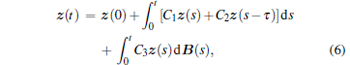 |
where the initial function is given by 
The last integral in Eq. (6) is a stochastic Riemann– Stieltjes integral, and Itô interpretation to the stochastic integral is naturally adopted in the following analysis.[26]
In order to derive the equation of first-order moment, we denote m(t) = Ez(t), and the DDE for m(t) is obtained by performing average on both sides of Eq. (6)
 |
with the initial condition 
Obviously, equation (7) is a deterministic DDE and its characteristic equation can be derived as
 |
From Refs. [11], [12], and [18], the first-order moment equation (7) with the characteristic equation (8) is delay-independent stable if and only if: (i) the function p(r, 0) is Routh– Hurwitz stable and (ii) the marginal stability condition p(iω , τ ) = 0 has no real solution ω for all given delays τ > 0.
According to Routh– Hurwitz criterion, the solutions of p(r, 0) = 0 are asymptotically stable if the following conditions are satisfied:
 |
Substituting r = iω (ω > 0) into Eq. ( 8) and separating the real part and imaginary part, one has
 |
Eliminating the harmonic terms in Eq. (10), one can write the following formula:
 |
where 
According to Ref. [12], equation (11) has no real root ω if the parameters satisfy the following condition:
 |
Theorem 1 The first-order moment of the interior equilibrium is delay-independent stable if and only if conditions (9) and (12) hold true.
However, condition (12) is unsatisfied in our model because of q ≤ 0. Equation (11) has one real root 
 |
That is, when condition (9) is satisfied, p(r, 0) = 0 is asymptotically stable. The first-order moment keeps stable until time delay τ ≥ τ 0 (here, τ 0 is determined by Eq. (13)).
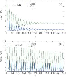
In the following, we choose the parameters as a = 1.5, b = 0.1, c = 0.6, d = 0.2, k = 0.4, m = 0.1 and the initial conditions (N0, P0) = (1.5, 0.5). It is obvious that condition (9) is satisfied under these chosen parameters. The first-order moment is zero-delay stable. When τ > 0, the first-order moment is stable if τ is less than the critical time delay τ 0 = 0.44. It is found that the interior equilibrium E* = (0.65707235, 3.141447) is asymptotically stable when τ = 0.42 < τ 0 (see Fig. 1(a)) and, then E* is unstable when τ = 0.51 > τ 0 (see Fig. 1(b)). In other words, the first-order moment is delay-dependent stable and the gestation period or reaction time of the predators plays an important role in the stability of the biological system.
 | Fig. 1. The time histories of system (2) with   |
In this section, we study the stability of the second-order moment E{z(t)zT(t)}. According to Itô ’ s differential rules and Eq. (5), we have

 |
 |
Let K(t, s) = Eu(t)u(s), R(t, s) = Eu(t)v(s), Q(t, s) = Ev(t)v(s), then the following formulas are satisfied:
 |
Then, equations (14)– (16) can be transformed into the following forms:
 |
 |
 |
For the Gaussian stationary process, the correlation function has the property of time-shift invariant. Thus, the approximation R(t − τ , t) = R(t, t − τ ) is used for small time delay in the following computation. The corresponding characteristic equation of Eqs. (18)– (20) is given by
 |
where
When τ = 0, equation D(r, 0, 0) = 0 is stable if and only if the following conditions hold:
 |
When τ > 0, substituting r = iω (ω > 0) into Eq. (21) and separating the real part and imaginary part, one has
 |
It is easy to find that function G(ω ) reads by eliminating the harmonic terms in Eq. (23),
 |
where
By using MAPLE routine discr, [12] one obtains the discriminant sequence of G(ω ) as follows:
 |
where
The expressions of dj (j = 5, … , 9) are not presented here because their expressions are lengthy.
Theorem 2 The second-order moment of the interior equilibrium is delay-independent stable if and only if: (i) condition (22) holds true; and (ii) the modified sign table of G(ω ) is subject to the condition l = 2s for s = 1, 2, … , n or 2n, where l and s are the numbers of non-zero terms and the number of variation of signs in the corresponding discrimination sequence, respectively.
When the second condition in Theorem 2 is unsatisfied, the second-order moment is delay-dependent stable. The polynomial G(ω ) has real roots and the corresponding critical time delays are derived as
 |
where
When condition (22) is satisfied, the second-order moment is zero-delay asymptotically stable for 


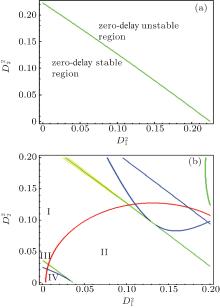
In Fig. 2, we plot the stable region for the second-order moment. The condition (22) holds true in the stable region as shown in Fig. 2(a). By plotting the graphs of di = 0 (i = 0, 1, … , 10), the region in the parameter space of 
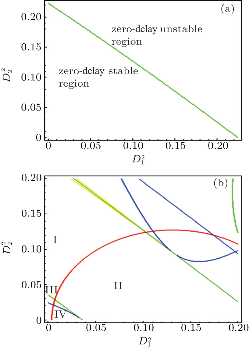 | Fig. 2. The delay-independent stable conditions for the second-order moment: (a) the first condition in Theorem 2; (b) the second condition in Theorem 2. |
| Table 1. Sign tables of the discrimination sequence (25). |
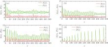
The effects of time delay on the stability of system solution in a stochastic delayed system (2) are shown in Fig. 3. It is seen that the oscillations of system solution increase with the increase of time delay. At last, the system becomes unstable. Figure 4 shows that the effects of noise intensities on the stability of the stochastic delayed system (2). It is obvious that oscillations of system solution increase with the increase of the noise intensities, which is consistent with the results obtained in Ref. [22]. Thus, the solution moment stability of stochastic delayed prey-predator model depends on time delay and noise intensity. Both first-order and second-order moments of system (2) are not delay-independent stable under this parameter combination. That is, the random fluctuation in the natural growth rate of the prey population and in the natural death rate of the predator population can destabilize the stochastic system (2).
 | Fig. 3. Time histories of model (2) with   |
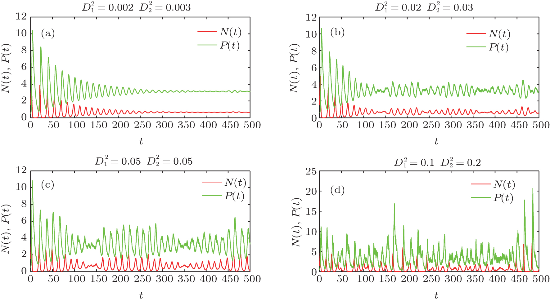 | Fig. 4. Time histories of model (2) with τ = 0.4 and different noise intensities. |
The random environmental fluctuation and time delay are common phenomena in real ecological systems. In this paper, the random fluctuations in both the growth rate of prey and the death rate of predator and the gestation time delay of predator have been considered in a Harrison-type functional response predator– prey model. In order to explore the effects of time delay on the stability of system solution, the delay-independent stable conditions of solution moments have been achieved in Theorem 1 and Theorem 2 by using the delay-independent stable criterion of a linear retarded system. It can be found that the first-order and second-order moments are delay-dependent stable under our chosen parameters and the critical time delays are given. That is, the stability of solution moments depends on time delay and environmental noise. Specifically, when the time delay exceeds the minimum critical time delay, the stability of the first-order and second-order moments will be broken with the increase of time delay and noise intensity. The gestation period or reaction time of the predators and environmental noise can also cause the instability of the predator– prey model. Thus, it is necessary to study the effects of time delay and noise on the dynamics of a predator– prey model.
| 1 |
|
| 2 |
|
| 3 |
|
| 4 |
|
| 5 |
|
| 6 |
|
| 7 |
|
| 8 |
|
| 9 |
|
| 10 |
|
| 11 |
|
| 12 |
|
| 13 |
|
| 14 |
|
| 15 |
|
| 16 |
|
| 17 |
|
| 18 |
|
| 19 |
|
| 20 |
|
| 21 |
|
| 22 |
|
| 23 |
|
| 24 |
|
| 25 |
|
| 26 |
|