
Direction-of-arrival estimation for co-located multiple-input multiple-output radar using structural sparsity Bayesian learning*
[Wen Fang-Qinga), b) , Zhang Gonga), b)  , Ben De
a), b), c) ]
, Ben De|
|


†Corresponding author. E-mail: gzhang@nuaa.edu.cn
*Project supported by the National Natural Science Foundation of China (Grant Nos. 61071163, 61271327, and 61471191), the Funding for Outstanding Doctoral Dissertation in Nanjing University of Aeronautics and Astronautics, China (Grant No. BCXJ14-08), the Funding of Innovation Program for Graduate Education of Jiangsu Province, China (Grant No. KYLX 0277), the Fundamental Research Funds for the Central Universities, China (Grant No. 3082015NP2015504), and the Priority Academic Program Development of Jiangsu Higher Education Institutions (PADA), China.
This paper addresses the direction of arrival (DOA) estimation problem for the co-located multiple-input multiple-output (MIMO) radar with random arrays. The spatially distributed sparsity of the targets in the background makes compressive sensing (CS) desirable for DOA estimation. A spatial CS framework is presented, which links the DOA estimation problem to support recovery from a known over-complete dictionary. A modified statistical model is developed to accurately represent the intra-block correlation of the received signal. A structural sparsity Bayesian learning algorithm is proposed for the sparse recovery problem. The proposed algorithm, which exploits intra-signal correlation, is capable being applied to limited data support and low signal-to-noise ratio (SNR) scene. Furthermore, the proposed algorithm has less computation load compared to the classical Bayesian algorithm. Simulation results show that the proposed algorithm has a more accurate DOA estimation than the traditional multiple signal classification (MUSIC) algorithm and other CS recovery algorithms.
The multiple-input multiple-output (MIMO) radar exploits multiple transmitting antennas to simultaneously transmit orthogonal waveforms, and utilizes multiple receiving antennas to receive the reflected signal. The information of an individual transmit path is extracted by a set of matched filters in the receiver, and the information from all the transmit paths enables the MIMO radar to achieve better performance than the traditional radars.[1] Theoretical research indicates that the MIMO radar has several built-in advantages in noise suppression, overcoming the fading effect, improving spatial resolution, enhancing parameter identifiability, etc.[2, 3]
Direction of arrival (DOA) estimation is a fundamental task in the MIMO radar that has been widely investigated in the past decades. However, most of the previous studies focused on the uniform array geometry, such as uniform linear arrays (ULA), uniform circular-shape, and L-shape arrays. To avoid phase ambiguity, elements in the uniform array geometry are spaced at intervals no larger than half wavelength of the transmit signal carrier. The uniform array setup, which performs spatial sampling at the Nyquist rate, requires the product of transmit and receive elements scale linearly with the array aperture. In addition, this kind of configuration leads to high volume of data, which may be more serious in a massive MIMO radar system.[4] Generally speaking, angle resolution improves with the increase of array aperture. For a given number of antenna elements, the minimum redundancy linear array (MRLA) can achieve the maximum resolution by reducing the redundancy of spatial correlation lags.[5] An MRLA configuration was introduced to the MIMO radar in Ref. [6] and achieved similar resolution with the ULA architecture. Compared with the MRLA configuration, the random array pattern provides a more flexible form for the MIMO radar, where transmit and receive elements are randomly placed over a large aperture and spatial sampling is applied at sub-Nyquist rate. The random array setup would achieve similar resolution with significantly fewer elements. Hence, the random array configuration has attracted much attention in recent years.[7]
DOA estimation for the random array architecture MIMO radar can be accomplished with a variety of algorithms. Classical angle estimation algorithms such as multiple signal classification (MUSIC)[8] estimate parameters via the spectral peak searching. The estimation method of signal parameters via rotational invariance techniques (ESPRIT)[9] utilizes the invariance property of both transmit array and receive array for angle estimation. The array in ESPRIT algorithm must be composed of two identical, translationally invariant sub-arrays. One main drawback of these algorithms is the necessity of processing singular value decomposition (SVD) or eigenvalue decomposition (EVD) of the received data, which requires the prior information of the incident signal number. Besides, large numbers of snapshots are necessary to ensure the stability of SVD or EVD, which is impractical for the fast-moving targets, as the direction of target is continuously changing over a period of time. As a result, only a few snapshots are available for DOA estimation. From a sparsity point of view, the number of targets in the detection background is much smaller than the total number of the interesting cells. Therefore, the angle estimation from the sub-sampled array data can be linked to a sparse inverse problem from multiple measurement vectors (MMV) in compressive sensing (CS), [10, 11] which can be solved by technologies such as basis pursuit (BP) algorithm, [12] orthogonal matching pursuit (OMP) algorithm, [13] FOCal underdetermined system solver (FOCUSS) algorithm, [14] and sparse bayesian learning (SBL) algorithm.[15] The motivation for sparse solution is to estimate the parameters more accurately compared to the traditional methods. Unfortunately, the complexity of BP algorithm is too high to implement. OMP and FOCUSS are sensitive to noise and have the problem of choosing a proper regularization parameter. As one important family of Bayesian algorithms, SBL has received much attention recently since it always achieves the sparsest global minima.[15] Besides, the statistical model in SBL provides a flexible framework to exploit special structures in the sparse signal, [16– 23] which may significantly improve the recovery performance.
Generally speaking, the special structures of the source matrix in the MMV model can be divided into two categories.[16] The first category is inter-correlation that describes the distribution of the nonzero entities in each column vector. The second category is intra-correlation that indicates the correlation between the entries in each of the non-zero rows. In Ref. [24], the intra-correlation was modeled with a zero-mean Gaussian process, and a maximum-likelihood estimator is derived for DOA estimation. To reduce the computational load in Ref. [24], a block Gaussian priori was present to describe the inter-cluster of the spatial power spectrum in array antenna DOA estimation.[25] The coarse locations of the sources were obtained via SBL, and a peak searching procedure was introduced for refined DOA estimation. A block Gaussian process was modeled in Ref. [26] to capture the intra-correlation of the incident sources, and the block sparse Bayesian learning (BSBL) was derived for the off-grid DOA estimation. The sparse representation coefficients in distributed MIMO radar were assumed to satisfy a parameterized multivariate Gaussian distribution in Ref. [27], and BSBL was exploited for multi-targets localization. These structures have been shown to be very effective in robust parameter estimation with limited snapshots. However, intra-block correlation was ignored by the previous literature, which may result in performance loss in the reconstruction.
This paper links the DOA estimation problem in random manifold configured co-located MIMO radar to support recovery in the CS framework. The intra-signal correlation of the received snapshots is modeled with a modified statistical model, which represents the correlation of the snapshots more accurately. The BSBL framework is introduced to exploit the special correlation. Angle estimation is then linked to hyperparameters learning in the Bayesian framework, and a low complexity Bayesian learning algorithm is developed to speed up the learning process. The proposed algorithm does not require the prior information of the target number, which means that our algorithm has blind and robust characteristic, therefore the proposed algorithm has higher working efficiency. The proposed algorithm has better DOA estimation accuracy than MUSIC method[8] and conventional CS methods. Besides, our approach reduces the computational cost of the conventional SBL algorithm.[15] Extensive experiments show the superiority of the proposed algorithm.
The rest of the paper is organized as follows. Section 2 presents the signal model for the spatial CS-MIMO radar and provides the proposed Bayesian algorithm. simulation results are given in Section 3. Finally, conclusion remarks are drawn in Section 4.
Notation Lower case and capital letters in bold denote, respectively, vectors and matrices. The superscripts (• )T, (• )H, (• )− 1, and (• )† represent the operations of transpose, Hermitian transpose, inverse, and pseudo-inverse, respectively; the subscripts | | • | | 0, | | • | | 1, | | • | | 2, and | | • | | F separately denote the l0-norm, l1-norm, l2-norm, and Frobenius norm, respectively; the vec(• ) operator stacks the columns of its matrix argument in one tall column; ⊗ and ⊙ represent the Kronecker product and Khatri– Rao product (column-wise Kronecker product).
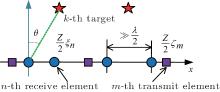
Consider the co-located MIMO radar model in Ref. [7], which is equipped with an M-element transmitter and an N-element receiver (as shown in Fig. 1). The transmitter and receiver are assumed to be linearly distributed in the x axis (possibly overlapping), with the total aperture ZTX and ZRX (normalized in wavelength units), respectively. The physical locations of the m-th transmitter and the n-th receiver are denoted by Zζ m/2 and Zξ n/2, respectively. Here, Z = ZTX + ZRX, ζ m lies in the interval [− ZTX/Z, ZTX/Z], and ξ n lies in the interval [− ZRXZ, ZRX/Z]. We assume that the transmitter antennas’ locations ζ are independent and identically distributed (i. i. d.) random variables governed by a distribution p(ζ ). Similarly, the positions of the receivers ξ are drawn i. i. d. from a distribution p(ξ ). It is also assumed that there are K non-coherent targets appearing in the far-field of the radar system, the DOA of the k-th target is denoted by θ k. Additional assumptions are that each transmit antenna emits a pulse train with L orthogonal waveforms, during which θ k is a constant and the effect of jammers and interference is compensated. The output of the matched filters at the n-th receiver can be expressed as
 |
where 


 | Fig. 1. MIMO radar system model. |
Define b(θ k) = [exp(jπ Zθ kξ 1), exp(jπ Zθ kξ 2), … , exp(jπ Zθ kξ N)]T ∈ CN× 1 as the steering vector of the receive array. Let the receive direction matrix B(θ ) = [b(θ 1), b(θ 2), … , b(θ K)], and the transmit direction matrix C(θ ) = [c(θ 1), c(θ 2), … , c(θ K)]. Arrange the matched filtering results as Y = [Y1, Y2, … , YN]T ∈ CMN× L with 
 |
where à (θ ) = B(θ ), … , C(θ ) ∈ CMN× K is the virtual array direction matrix, S = [S1, S2, … , SL] ∈ CK× L with 
It is assumed that the targets are located in the maximum unambiguous angles. By discretizing the possible target DOA on a fine uniform grid, i.e., [φ 1, φ 2, … , φ G](K ≪ G), we can obtain an over-complete dictionary 
 |
where Xg• denotes the g-th row vector of matrix X. Our aim is to recover θ from the given measurements Y and the known matrix 

DOA estimation problem from Eq. (3) is equivalent to supporting recovery from the received array data, which can be accomplished by solving the following non-convex l0-norm problem:
 |
where | | X| | 0 is a row-diversity measure which counts the number of nonzero rows in X, and ε represents the noise level. The cost function (4) can be globally minimized using a variety of optimization algorithms. However, as MN ≪ G, the linear system in Eq. (3) is highly underdetermined and equation (4) is usually NP-hard. CS theory has pointed out that under specific conditions, [11] the l0-norm optimization problem can be approximated by its l1-norm relaxation with a bounded error, which is expressed as
 |
Since the noise is present, the solution is decidedly nebulous. In practice, equation (5) is always transformed into an unconstrained regularized formulation and accomplished with an alternative strategy, suggesting the relaxed optimization problem
 |
where η is a tradeoff parameter balancing the estimation quality. The regularization term 𝔍 (X) denotes the essential diversity measure, and it varies with the algorithm. When 
The key idea of applying Bayesian framework to recover the row sparse signal X is to establish a hierarchical prior in X. We assume that all sources Xg• (g = 1, 2, … , G) are mutually independent, thus the inter-signal correlation in of the source is assumed to be an independent Gaussian process. We assign a structural prior on Xg• , the density of Xg• is therefore given by
 |
where N(0, γ gRg) represents the Gaussian distribution with zero mean and covariance γ gRg. In this prior model, γ g is a hyperparameter, Rg is the covariance matrix of Xg• . Hence, the inter-signal correlation of the source is modeled with a parameterized multivariate Gaussian process. The non-negative hyperparameter γ g controls the row sparsity of Xg• , i.e., γ g = 0, the associated Xg• becomes zeroes. Unlike the block sparse model in Ref. [21], the added positive matrix Rg captures the intra-block correlation of Xg• and needs to be estimated.
We construct the following vectors: y = vec(YT), x = vec(XT), and n = vec(ET). Let 
 |
We postulate n to be i.i.d. zero mean Gaussian variable with variance λ , i.e., p(n) ∼ N(0, λ ). As a result, the likelihood function for y in Eq. (8) could be formulated as
 |
which is consistent with the likelihood model implied by Eq. (6) and previous Bayesian methods. To simplify the model, we just assume that all the sources have the same correlation structure, i.e., R1 = R2 = · · · = RG = R. We define 
 |
where det (Γ ) denotes the determinant of matrix Γ . By using the Bayes rule, the posterior probability function for x can be derived from Eqs. (9) and (10), which is also Gaussian and given by
 |

with mean and covariance given by
 |
Subsequently, to obtain the posterior probability function in Eq. (11), we have to estimate the hyperparameters λ , 
 |
where Φ = λ I + Θ Γ Θ T. To obtain the hyperparameter λ , the EM method proceeds by treating 
 |
where 
 |
where λ d, xd, Σ d, and Γ d are previously obtained estimates of λ , x, Σ , and Γ , respectively. similarly, to obtain the hyperparameters 
 |
Taking the gradient of Eq. (16) with respect to 

 |
where μ d, Σ d, and Rd are previously obtained estimates of μ , Σ and R, respectively. By treating 

 |
where μ d, Σ d, and (γ q)d are previously obtained estimates of μ , Σ , and γ q, respectively. The algorithm using iterative learning rules (12), (15), (17), and (18) is denoted by block SBL.
BSBL was proved to provide highly accurate solutions. However, it suffers from high computational complexity, as the vec(• ) operator maps the inverse problem to a higher-dimensional space. To speed up the learning process of block SBL, we map the learning of the parameters in a higher-dimensional space to the original problem. The mean and covariance in Eq. (12) are updated using the rules in MSBL method[15]
 |
where 
 |
 |
 |
where η is a positive scalar. The faster version is very similar to that of MSBL method. The only difference is the added R in 
Till now, we have achieved the proposal for the structural sparsity Bayesian learning based on the DOA estimation algorithm in the MIMO radar. The major steps of the proposed algorithm are shown as follows.
1) Initialize X to a matrix that elements are all 1, initialize R to an identity matrix, set λ = 10− 6 and set the iteration count d = 0.
2) Subsequently, solve the MMV minimization problem by alternatively iterating among Eqs. (20)– (22).
3) Afterwards, compute the posterior moments X and Σ X using Eq. (19).
4) Repeat Eqs. (2) and (3) until convergence or the iteration count d attains a specified maximum number.
In this section, Monte Carlo simulations are used to assess the DOA estimation performance of the proposed algorithm. Success-rate and average running time are used for performance evaluation. A successful trial is recognized if the indexes of estimated sources with the K largest l2-norms are the support of X. In our simulation, the total aperture of the elements is Z = 250. It is assumed that targets are located in the far field, and the RCS coefficients of each target satisfy the first-order autoregressive process with the correlation coefficient β = 0.9. In our experiments, we compare our algorithm with the traditional MUSIC algorithm and the following CS recovery algorithms for the MMV model: the MOMP method proposed in Ref. [13], the MFOCUSS algorithm proposed in Ref. [14], and the MSBL method proposed in Ref. [15], which could be regarded as a faster version of the BSBL method. The computer used to run the simulation is a HP Z400 workstation, which is configured with four Intel Xeon W3550 3.07 GHz processors, and 12 GB of RAM.
Figure 2 depicts the DOA estimation performance comparison of all the algorithms with L = 5, M = N = 6, θ = [15, 40, 65] and different values of SNR in the numerical simulations. According to Fig. 2, all algorithms would achieve better performance with the increase of the SNR. It is obvious that the proposed algorithm could provide almost precise results. Notably, compared with the MSBL method, our algorithm has better DOA estimation accuracy at low SNR, and the proposed algorithm is appealing from the running time point of view, since more precision of the estimated temporary variables would result in much fewer learning steps. As shown in this figure, the MOMP method possesses poor success rate. This is caused by the severe mutual coherence between the atoms of the dictionary 
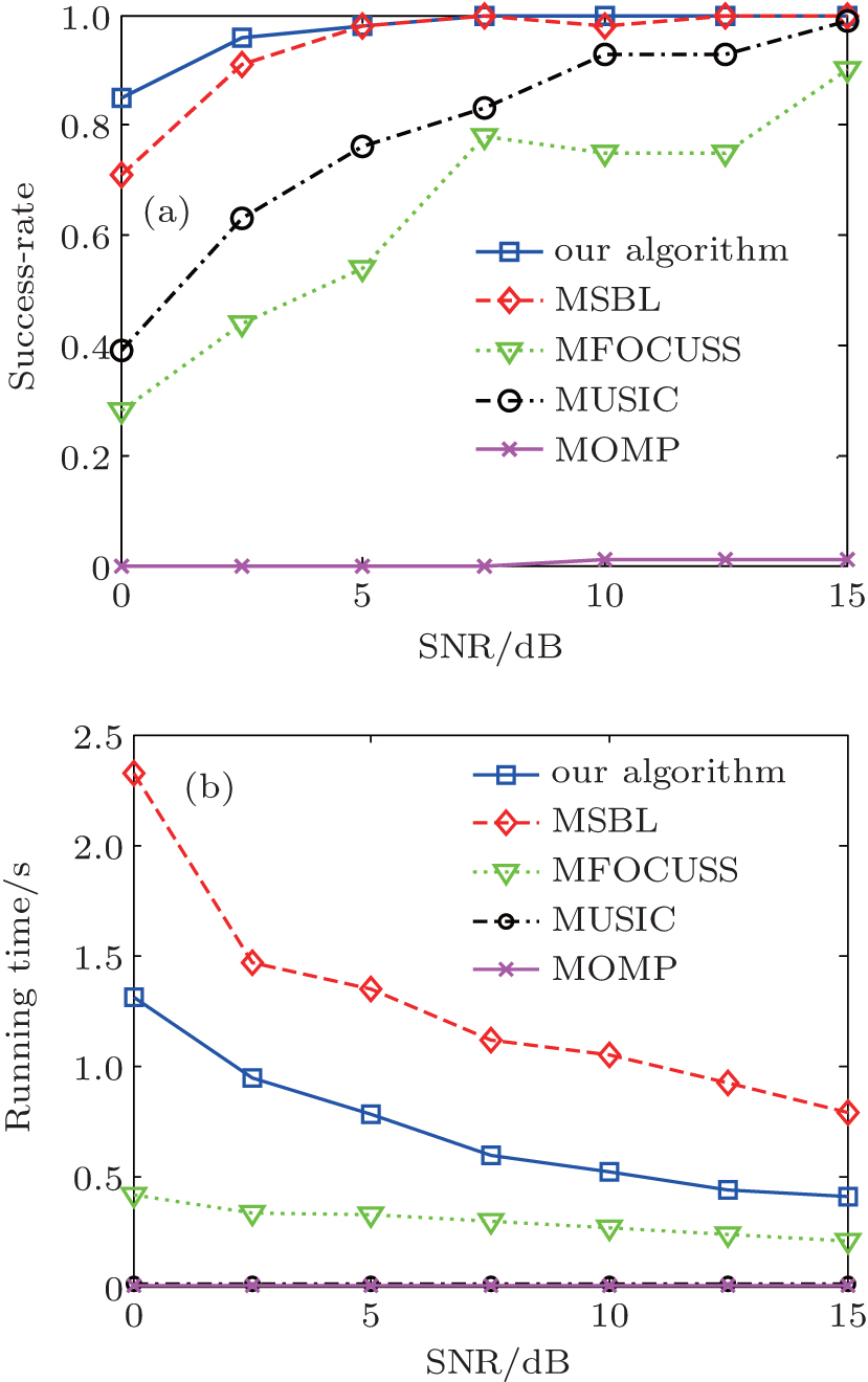 | Fig. 2. Performance of all the algorithms with different SNR. (a) Success-rate comparison and (b) average running time comparison. |
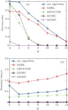
The DOA estimation performance comparison of all the algorithms with respect to different sparsity K was investigated in the simulation, as shown in Fig. 3. Therein, M = N = 6, L = 5, and SNR = 10 were considered in the simulation. In each trial, the locations of the targets were randomly uniformly chosen from the feasible regions 0° – 90° . It is clearly shown that the Bayesian algorithm accurately recovers much more targets than other algorithms. Thanks to the learning process of the intra-block correlation parameter, the proposed algorithm performs better than the MSBL method.
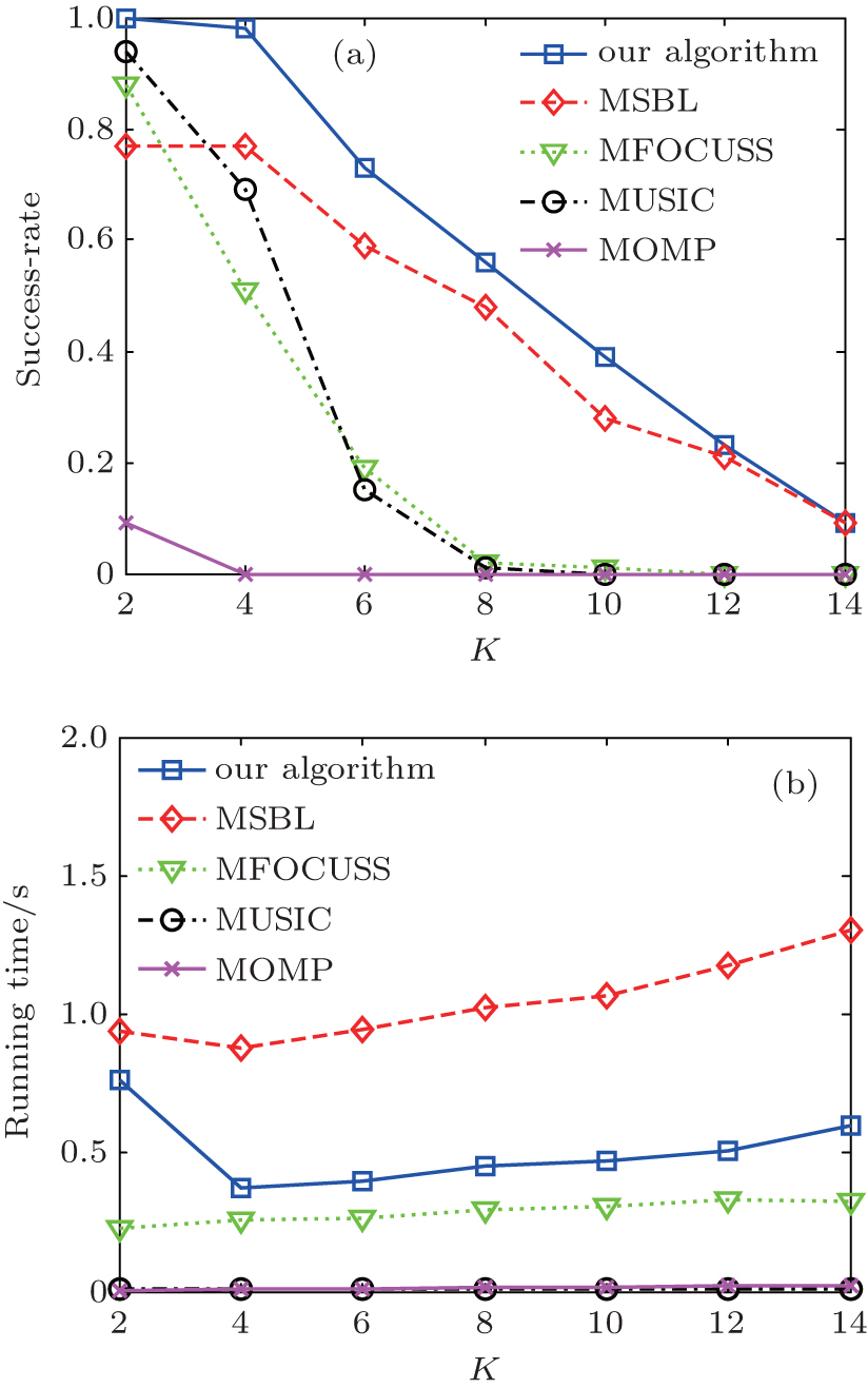 | Fig. 3. Performance of all the algorithms with different sparsity K. (a) Success-rate comparison and (b) average running time comparison. |
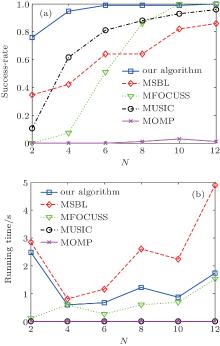
Figure 4 shows the DOA estimation performance comparison of all the algorithms with different number of receive antenna N, where M = 6, L = 5, θ = [15, 40, 65], and SNR = 10. It indicates that angle estimation accuracy of all the algorithms were improved with N increasing. The proposed algorithm requires significantly fewer numbers of antenna for the same successful enumeration, and only requires about 5 receive antennas to start stabilizing (success-rate more than 95%). simulation results are consistent with CS theory, which indicates that recovery performance would rapidly be improved with the increase of the measurement length, as more measurements would provide more information for the sparse recovery.
 | Fig. 4. Performance of all the algorithms with different antenna number N. (a) Success-rate comparison and (b) average running time comparison. |
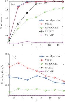
Figure 5 illustrates the angle estimation performance comparison of all the algorithms with different snapshots L, where M = N = 6, θ = [15, 40, 65], and SNR = 10. Figure 5(a) shows clearly that the increasing number of snapshots improves the estimation resolution. However, once L reaches a value (approximately equal to 5 in our simulation), the benefit from MMV becomes indistinct. Therefore, an appropriate number of snapshots is important for the proposed algorithm, as a smaller L value may impair the angle estimation accuracy, and large L values may require more computational resources.
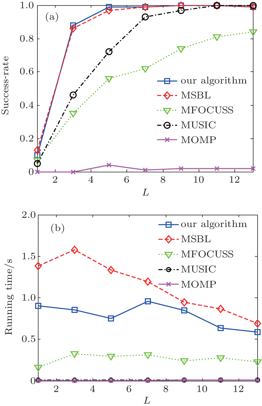 | Fig. 5. Performance of all the algorithms with different snapshot L. (a) Success-rate comparison and (b) average running time comparison. |
In this paper, we have proposed a structural sparsity Bayesian model for DOA estimation in the spatial CS MIMO radar. Our work links the DOA estimation problem to the parameters learning in the Bayesian framework, which significantly reduces the computation load of conventional Bayesian algorithm. The proposed algorithm requires no prior information of the number of targets, and achieves DOA estimation performance better than the traditional Bayesian algorithm. The proposed algorithm outperforms the traditional MUSIC algorithm and other CS recovery algorithms with fewer numbers of snapshots and low SNR scene.
| 1 |
|
| 2 |
|
| 3 |
|
| 4 |
|
| 5 |
|
| 6 |
|
| 7 |
|
| 8 |
|
| 9 |
|
| 10 |
|
| 11 |
|
| 12 |
|
| 13 |
|
| 14 |
|
| 15 |
|
| 16 |
|
| 17 |
|
| 18 |
|
| 19 |
|
| 20 |
|
| 21 |
|
| 22 |
|
| 23 |
|
| 24 |
|
| 25 |
|
| 26 |
|
| 27 |
|