


Flexible reduced field of view magnetic resonance imaging based on single-shot spatiotemporally encoded technique
[Li Jinga) , Cai Cong-Bob) , Chen Lina) , Chen Yingc) , Qu Xiao-Boa) , Cai Shu-Hui†a)  ]
]
]
|
|


†Corresponding author. E-mail: shcai@xmu.edu.cn
*Project supported by the National Natural Science Foundation of China (Grant Nos. 11474236, 81171331, and U1232212).
In many ultrafast imaging applications, the reduced field-of-view (rFOV) technique is often used to enhance the spatial resolution and field inhomogeneity immunity of the images. The stationary-phase characteristic of the spatiotemporally-encoded (SPEN) method offers an inherent applicability to rFOV imaging. In this study, a flexible rFOV imaging method is presented and the superiority of the SPEN approach in rFOV imaging is demonstrated. The proposed method is validated with phantom and in vivo rat experiments, including cardiac imaging and contrast-enhanced perfusion imaging. For comparison, the echo planar imaging (EPI) experiments with orthogonal RF excitation are also performed. The results show that the signal-to-noise ratios of the images acquired by the proposed method can be higher than those obtained with the rFOV EPI. Moreover, the proposed method shows better performance in the cardiac imaging and perfusion imaging of rat kidney, and it can scan one or more regions of interest (ROIs) with high spatial resolution in a single shot. It might be a favorable solution to ultrafast imaging applications in cases with severe susceptibility heterogeneities, such as cardiac imaging and perfusion imaging. Furthermore, it might be promising in applications with separate ROIs, such as mammary and limb imaging.
The last decades have witnessed a continuous growth in the use of single-shot MRI, both for clinical and research applications.[1– 8] Owing to the good temporal resolution, these single-shot MRI methods are referred to as “ ultrafast” imaging protocols. These “ ultrafast” protocols play an essential role in experiments and researches demanding high temporal resolution.[1, 2, 5– 7] Single-shot echo planar imaging (EPI) is one of the most popular of these ultrafast imaging protocols.[9– 11] For single-shot EPI, full k-space lines are collected in a single shot to reduce the acquisition time. However, the extremely long echo-train length (ETL) in EPI reduces the image quality due to the occurrences of ghosts, ringing artifacts, geometric distortion, etc.[12– 16] The reduction of the total echo-train duration can be accomplished by reducing the ETL; however, it does so at the expense of spatial resolution. In many ultrafast imaging applications, reduced field-of-view (rFOV) imaging technique can be used to reduce the number of phase encoding lines and, hence, reduce the ETL without compromising spatial resolution for those applications in which the region of interest (ROI) is only a small part of the field of view (FOV).[11, 17– 22]
Several rFOV imaging techniques have been proposed, including spatial pre-saturation, [12, 17] orthogonal RF excitation, [23] and two-dimensional (2D) spatially selective RF (2DRF) pulses excitation.[18, 21] Spatial pre-saturation is usually sensitive to B1 inhomogeneity, although some techniques have been used to improve the B1 inhomogeneity tolerance.[12, 17] For pulse sequences with long repetition time (TR) such as spin-echo EPI, another problem associated with spatial pre-saturation is that the T1 recovery of the transverse magnetization in the saturation region during acquisition usually degrades saturation performance. For the rFOV imaging method using orthogonal RF excitation and 2DRF pulses excitation, the aliasing artifacts will be generated if the excited area is larger than the imaged rFOV, [18, 21, 23] especially in inhomogeneous fields.
Recently, a single-shot spatiotemporally-encoded (SPEN) MRI approach has been proposed.[24– 26] This approach uses a linear frequency-modulated pulse (chirp pulse) and a simultaneous linear gradient field to sequentially excite the nuclear spins along the direction of the gradient with a quadratic phase profile, and the MRI signals are then acquired in the same way as traditional EPI methods. The quadratic phase profile focuses the signal from a region around its vertex where all the spins are in-phase, while largely suppressing the signals from other regions where the spins destructively interfere with each other. Therefore, the SPEN method possesses a space-selective property. It offers a novel approach for single-scan imaging, which can alleviate the influences of field inhomogeneities and chemical shift but which possesses comparable temporal resolution with EPI.[24, 26] Meanwhile, the stationary-phase characteristic and band-selective excitation of SPEN method offer an inherent ability to rFOV imaging.[22, 27– 29] It has been mentioned that two or more separated ROIs can be locally imaged by using single-shot biaxial SPEN (bi-SPEN) MRI sequence, [22] which utilizes a 90° chirp pulse and a 180° chirp pulse incorporated with two orthogonal gradients to spatiotemporally encode two dimensions (i.e. high-bandwidth dimension and low-bandwidth dimension) and a series of suitably tailored decoding gradients to acquire the signals from the spins in ROIs. Since two chirp pulses (especially the 180° chirp pulse) are used for the spatiotemporal encoding, the bi-SPEN sequence may cause high specific absorption ratio (SAR).[26] Moreover, the principle of the flexible ROI imaging and performance of this method have not been discussed in detail in the previous report. To reduce the SAR and image two or more ROIs with high spatial resolution in a single shot, we present a flexible rFOV imaging method in this paper based on the single-shot SPEN MRI sequence. This method can not only scan any one ROI along the SPEN direction but also scan two or more separated ROIs in a single shot. Meanwhile, we analyze the method by introducing a parameter P. The performances of this method in signal-to-noise ratio (SNR), SAR, and immunity to the B0 inhomogeneity are discussed.
This paper is organized as follows. In Section 2, we carry out a theoretical derivation for the present method. Meanwhile, we discuss the performance of this method in SNR, SAR and immunity to the B0 inhomogeneity. In Section 3, we show the performance of this method in SNR, flexible imaging and immunity to the inhomogeneous field through phantom and in vivo experiments. In Section 4, we discuss some related issues experimentally. Finally, in Section 5, we draw some conclusions from this study.
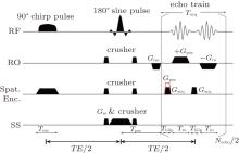
For simplicity, a one-dimensional (1D) imaging along the y direction is taken as an example to illustrate the principle of the proposed flexible rFOV imaging scheme. The pulse sequence is shown in Fig. 1. Unlike the previous fixed rFOV method proposed by Chen et al., [28] an additional positioning gradient Gpos is used to flexibly image the region of interest (ROI) along the SPEN dimension. In the single-shot SPEN imaging, spatiotemporal encoding is realized by a π /2-chirp pulse combined with an encoding gradient Gexc along the y direction during the excitation period Texc.[24– 26] A quadratic y-dependent phase profile, which is imposed on the spins after excitation, can be written as follows:[24, 26]

where γ is the gyromagnetic ratio, Ly is the encoded FOV. Gexc is determined by

where Δ OHz is the bandwidth of the chirp pulse in units of Hz and R = Δ OHz/Texc is the frequency sweep rate in units of kHz/ms.
 | Fig. 1. 2D SPEN sequence with flexible rFOV scheme used in this study. The 180° pulse is used for slice selection and refocusing. Gexc is the encoding/exciting gradient, Texc is the encoding time, Gacq is the decoding/sampling gradient, Gpos is the positioning gradient transferring the current decoding location to the start location of next ROI, Tpre is the pre-acquisition delay, and Tacq is the decoding time (Tacq = Necho · Tblip, where Necho is the number of sampling points along the SPEN dimension, Tblip is the duration of one blip gradient along the SPEN dimension). Notice that Gpos is applied only when the decoding position needs to be transferred to the next ROI. In other cases, it is replaced by the decoding gradient Gacq. Abbreviations: exc: spatiotemporal-encoding excitation, ro: readout direction, acq: acquisition, echo: sampled echoes, blip: blip gradient, pos: position, pre: pre-acquisition, and ror: rephased gradient. |
During the acquisition/decoding period Tacq (Tacq = Necho· Tblip), an additional phase term

is added to Eq. (1). Therefore, the acquired signal s(ta) can be expressed as
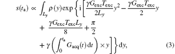
where ρ (y) represents the spin density. Given the quadratic y-dependence of φ exc, the spins phase will vary rapidly across the sample, [24, 26] except at a single stationary phase point where the first spatial derivative of the overall phase vanishes: (∂ /∂ y) [φ all (y, ta)] = 0.[24– 26] According to this stationary-phase approximation, only the spins in close vicinity of this time-dependent y point will have in-phase magnetizations and contribute to the acquired signal s(ta).[24– 26] The decoded trajectory (y′ ) at decoding time (ta) can be obtained from.[30, 31]
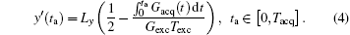
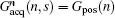
According to Eq. (4), the decoded position can be shifted flexibly along the y direction (i.e. the SPEN dimension) via suitably tailoring the gradient Gacq(t).[22] The gradient Gacq(t) is a general representation, and actually consists of positioning gradient Gpos and decoding gradient Gacq in the flexible rFOV imaging Assume that there are N ROIs along the SPEN dimension then 

where Gacq(n, s) is the discrete form of Gacq(t), Gpos(n) is the positioning gradient of the n-th ROI, 

Consequently, we have the discrete form of Eq. (4) as follows:
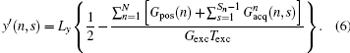
From Eq. (6), the decoded/imaged FOV of the n-th ROI can be defined as
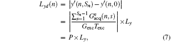
where

(P is a real number). From Eq. (7), we can find that FOV Lyd(n) can be determined by the sum of 

then a decoded/imaged FOV Lyd(n) smaller than the excited/encoded FOV (Ly) can be obtained. Note when P = 1 and N = 1, i.e. Sn = Necho, Ly = Lyd, and

the imaging scheme returns to the fixed rFOV imaging. For the fixed rFOV imaging, according to Eq. (2), scanning a smaller FOV with the same matrix size as a full FOV requires larger excitation/encoding and acquisition/decoding gradients. From Eq. (7), we can see that imaging a smaller FOV can be realized by reducing P, i.e., reducing 
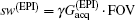
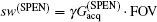
High SNR usually benefits single-shot MRI in clinical applications. The SNR of k-space encoded EPI and SPEN MRI can be compared by[25]

where 

Another important aspect in MRI application relates to SAR limitation. Owing to the gradient involved in the chirped excitation in the SPEN imaging, the accompanying frequency sweep RF pulse requires a higher bandwidth than the normal slice selective pulses used in traditional k-space encoded imaging. A high excitation bandwidth can enhance the robustness of the image to the B0 inhomogeneity but reduce the SNR. On the other hand, as reported previously, the SAR in SPEN MRI can be expressed as[26]

Equation (9) shows that a high excitation bandwidth Δ OHz of chirp pulse will lead to a high SAR. Therefore, the selection of excitation bandwidth is a compromise and should be carefully set in actual experiments.
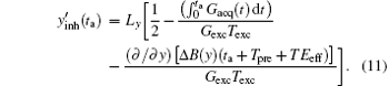
The above mentioned contents were discussed based on the assumption that all field inhomogeneity effects were negligible. Here, we discuss the behavior of the proposed rFOV imaging method in inhomogeneous fields. For simplicity, we focus on the effect of field inhomogeneity along the y direction during acquisition period and assume that there is only one ROI to be imaged. When a field inhomogeneity Δ B(y) exists, the final acquired signal can be expressed as the following integral:[22]
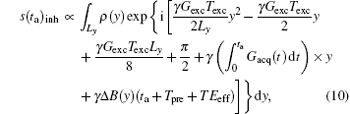
where Tpre is the pre-acquisition delay and T Eeff is the effective echo time. For the SPEN sequence shown in Fig. 1, the T Eeff for the spins in position y can be expressed as T Eeff = (yTexcy/Ly − T E/2), and the sign of T Eeff is always negative in this study because Texc is smaller than T E (see Fig. 1).[22] Because the evolution times for spins in different positions along the y direction are different, T Eeff values are different for spins at different positions, depending on the excitation instant.
According to the principle of the SPEN MRI, the stationary phase point under the B0 inhomogeneous field can be found by calculating the spatial derivative of the overall phase, and the real time decoding trajectory 
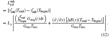
Assume that the decoding time varies from Tbegin to Tend, the final imaged/decoded FOV 
According to Eq. (12), the terms induced by Δ B(y) can be extracted as follows:
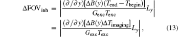
where Δ FOVinh represents the deviation of FOV affected by the B0 inhomogeneous field and Δ Timaging is the imaging time for decoding the ROI. For the proposed flexible rFOV imaging method, the excitation/encoding gradient Gexc and the acquisition/decoding Gacq satisfy P · | GexcTexc| = | GacqTacq| (P < 1). Therefore, equation ( 13) can be transformed to
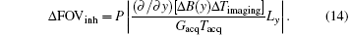
From Eq. (14), we can learn that the degree of distortion, Δ FOVinh, is directly proportional to the imaging time Δ Timaging and is inversely proportional to the acquisition/decoding time. Namely, a longer time to image the ROI and a smaller acquisition/decoding Gacq will lead to a more serious distortion. Therefore, when the acquisition/decoding Gacq used in the flexible SPEN rFOV imaging is equal to or smaller than the one used in EPI, the resulting SPEN image may become as sensitive to the B0 inhomogeneity as EPI; or even more, of course, with an improved SNR. Note that when the flexible FOV method is applied in vivo, the excitation bandwidth should be chosen carefully to retain the robustness of the method to the B0 inhomogeneity.
The MRI experiments were carried out with the single-shot sequence depicted in Fig. 1. In this sequence, the frequency encoding and spatiotemporal encoding were applied along two orthogonal axes, respectively, while the slice selection along the third axis was achieved by a 180° refocusing pulse. To evaluate the flexible rFOV imaging method with different values of P, the rFOV results were compared with those obtained with the single-shot EPI method with orthogonal RF excitation. For single-shot MRI sequences, including EPI sequence and SPEN sequence, the vertical axis was phase-encoded/SPEN dimension and the horizontal axis was traditional frequency-encoded dimension unless otherwise specially stated. For a fair comparison, the images obtained with SPEN and EPI sequences had the same matrix size. Moreover, SNR comparisons of different imaging methods were also given for in vivo rat brain experiments. The SNR value was measured as SNR = 10log [Mean(signal2)/Var(noise)], where Mean(signal2) denoted the average signal power of signal region and Var(noise) referred to the noise intensity variance of background region. In Fig. 2(c), the signal region is circumscribed with a rectangle in the rat head region and the noise regions are circumscribed with two rectangles in the black background region close to the edges of the image. The unit of SNR was dB. For each experiment, detailed experimental parameters were given in the captions of relevant figures. The displayed results were super-resolved (SR) enhanced images (see Appendix A2 for SR reconstruction). All of the images shown in this study were images after interpolation and the matrix sizes of all the images were also given in each figure caption. For the representation of sampling data matrix size or imaging matrix size m × n, m represented the size along the horizontal axis and n referred to the size along the vertical axis, unless otherwise specified. The imaging matrix was obtained by applying interpolation to the sampling matrix during SR reconstruction.
 | Fig. 2. Imaging results of a sagittal plane of an in vivo rat head. Slice thickness = 2 mm, imaging matrix size = 256 × 256, Lx = 60 mm (horizontal), Ly = 60 mm [(a)– (c)], 20 mm [(d)– (f)] (vertical). (a) and (d) EPI images (sampling data matrix size = 64 × 64, Gacq = 0.0196 T/m (a), 0.0367 T/m (d), sequence execution time = 47.6 ms). (b) and (e) SPEN images (P = 1, Gacq = 0.0367 T/m (b), 0.0587 T/m (e)). (c) Reference multi-scan gradient echo image (sampling data matrix size = 128 × 128, repetition time (TR) = 100 ms, dummy scans = 16, sequence execution time = 14.4 s). (f) SPEN image obtained with the flexible rFOV imaging method (P = 0.625, Gacq = 0.0311 T/m). Common parameters for SPEN imaging: Texc = 3 ms, Δ OHz = 64 kHz, sampling data matrix size = 64 × 64, R = 21.3 kHz/ms, sequence execution time = 49.1 ms, and acquisition bandwidth along readout dimension = 250 kHz. |
The flexible rFOV imaging method was also tested in rat cardiac imaging and perfusion imaging. These experiments were chosen to showcase the capabilities of the flexible rFOV imaging method in challenging cases with severe susceptibility heterogeneities as well as to prove the potential of the method to be a real-time imaging tool. In the cardiac imaging, a series of images depicting different heart beating stages was captured without ECG-triggering, respiratory gating, or breath holding. In perfusion imaging, a rat was injected with poly(aspartate acid & phenylalanine)-DOTA-Gd (PL-DF-DOTA-Gd), where DOTA-Gd was the abbreviation of 1, 4, 7, 10-tetraazacyclododecane-1, 4, 7, 10-tetraacetic-acid-gadolinium. After the rat was anesthetized and the imaging experiments began, it was injected over about 1 min with the contrast agent. Four thousand images were acquired over 80 min for each perfusion imaging experiment and the time courses were drawn from the resulting images for selected pixels.
In vivo imaging experiments were carried out on several Sprague-Dawley rats of seven-weeks old. The experiments were performed in accordance with the procedures approved by the Animal Experimental Center of our university. Before the experiments, the rats were anesthetized. The experiments were performed at 298 K on a 7.0-T Varian MRI system with a horizontal-bore Magnex magnet, equipped with 10 cm bore imaging gradients (40 Gs/cm) (Agilent Technologies, USA). The unit 1 Gs = 10− 4 T.
The results of the rat head are given in Fig. 2 to compare the SNR and image quality of different methods. They indicate that the SPEN sequence can produce images with good quality, even in areas where conventional EPI sequence is incompetent due to severe susceptibility heterogeneities (Fig. 2(a) versus Fig. 2(b)). The rFOV imaging improves the spatial resolution and immunity to field inhomogeneities of both EPI and SPEN images. However, the SNR is reduced compared with the corresponding full FOV image because the acquisition bandwidth is enlarged with the increasing of decoding/acquisition gradient strength, which leads to large noises. Note that the SNR of rat head image acquired by the proposed method with P = 0.625 is 38.5 dB, which is the highest among the rFOV images with the same FOV. This is because the image obtained using the flexible SPEN method is acquired with lower acquisition gradients than those obtained using other methods. It should be noted that when the acquisition gradients are lowered, the spatial resolution of the resulting image will be affected by smoothing the image to some extent. Therefore, the acquisition gradients need to be carefully set in the SPEN experiments.
The results of phantom and rat head are given in Figs. 3 and 4, respectively, to show the performance of the flexible imaging method. Compared with the SPEN images (Figs. 3(c) and 4(c)), EPI images (Figs. 3(b) and 4(b)) show much more serious geometric distortions and even have aliasing artifacts (e.g. Fig. 4(b)). It can be seen from Figs. 3(d)– 3(f) that any ROI along the SPEN dimension can be rFOV imaged by the proposed method and the rFOV images possess better spatial resolution than the full FOV images, including the EPI image (Fig. 3(b)) and the SPEN image (Fig. 3(c)). However, these rFOV images exhibit severer geometric distortions than the full FOV SPEN image (Fig. 3(c)). This is because much more imaging trajectories travel inside the target imaging region, and the influence of local inhomogeneous field is greater because of longer imaging time and smaller decoding gradients. Two separated ROIs can be rFOV imaged in a single shot and the resulting phantom image (Fig. 3(g)) and rat head image (Fig. 4(d)) show better quality in the aspect of spatial resolution and geometric shape than the EPI images (Figs. 3(b) and 4(b)), such as the region pointed by white arrow in Fig. 4.
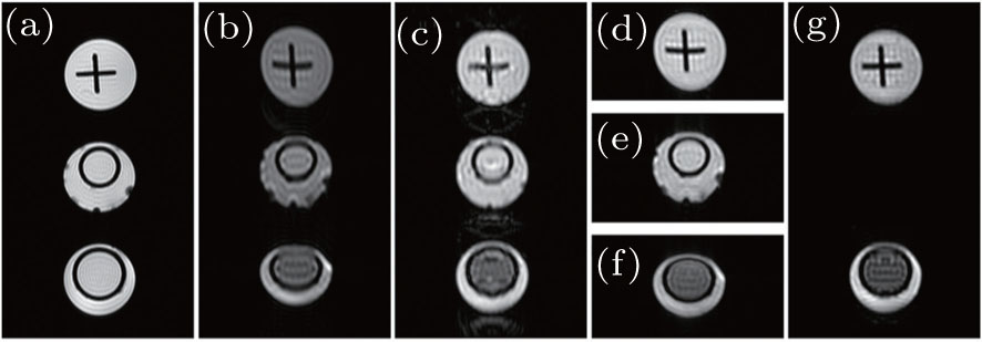 | Fig. 3. Imaging results of water phantom. Slice thickness = 2 mm, imaging matrix size = 256 × 256, Lx = 40 mm (horizontal), Ly = 70 mm [(a)– (c)], 23 mm [(d)– (f)], 46 mm (g) (vertical). (a) Reference multi-scan gradient echo image (sampling data matrix size = 256 × 256, dummy scan = 32, TR = 600 ms, sequence execution time = 172.8 s). (b) Full FOV EPI image (sampling data matrix size = 64 × 64, Gacq = 0.0168 T/m, sequence execution time = 47.6 ms). (c) Full FOV SPEN image (P = 1, Gacq = 0.0756 T/m). (d)– (f) The rFOV image obtained with flexible decoding scheme for different ROI (P ≈ 0.3, Gacq = 0.0252 T/m). (g) The rFOV image obtained with flexible decoding scheme for two ROIs (P ≈ 0.7, Gacq = 0.0504 T/m). Common parameters for SPEN imaging: Texc = 3 ms, Δ OHz = 96 kHz, sampling data matrix size = 64 × 64, R = 32 kHz/ms, sequence execution time = 49.1 ms, and acquisition bandwidth along readout dimension = 250 kHz. |
 | Fig. 4. Imaging results of a coronal plane of an in vivo rat head. Slice thickness = 2 mm, imaging matrix size = 256 × 256, FOV = 50 (horizontal) × 60 (vertical) mm2. (a) Reference multi-shot fast spin-echo image (sampling data matrix size = 256 × 256, sequence execution time = 544 s). (b) EPI image (sampling data matrix size = 64 × 64, sequence execution time = 49.6 ms). (c) SPEN image (P = 1). (d) SPEN image obtained with flexible rFOV method for two ROIs (P = 0.7, each ROI Lyd = 20 mm). Common parameters for SPEN imaging: Texc = 27.1 ms, Δ OHz = 7.1 kHz, sampling data matrix size = 64 × 64, sequence execution time = 59.1 ms, R = 0.26 kHz/ms, and acquisition bandwidth along readout dimension = 250 kHz. |
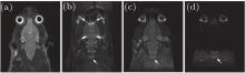
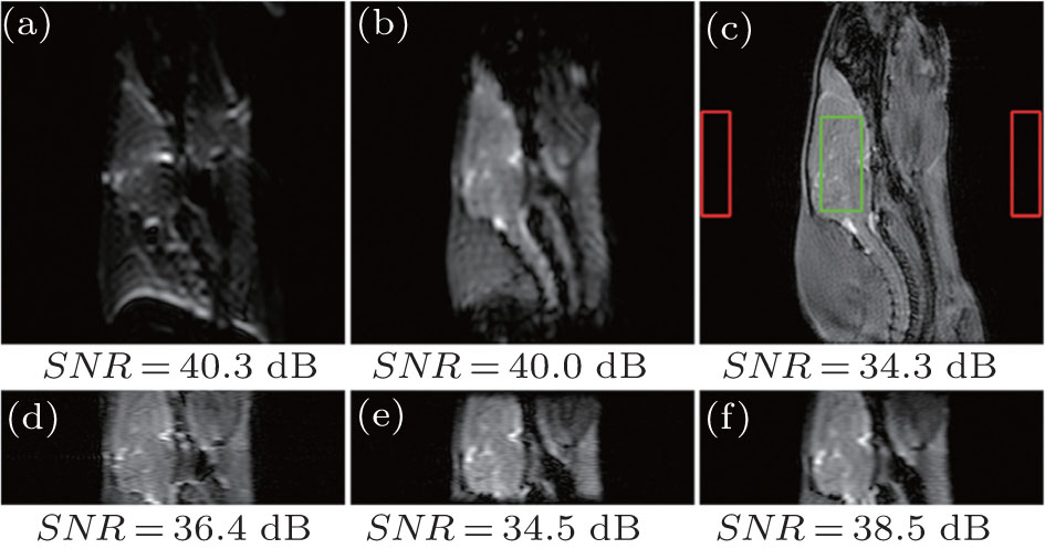
Figure 5 shows the results of rat cardiac imaging. It can be seen that the MR signal of blood is lost because of the short cardiac cycle and large blood flow velocity. Therefore, all of the rFOV images shown in Fig. 5 display the black blood contrast. The rFOV EPI images shown in Fig. 5(a) display severer geometric distortions than the flexible rFOV SPEN images (Fig. 5(c)) around the interfaces of tissue and air, e.g. the region pointed by white arrow in Fig. 5. Moreover, the rFOV EPI images are spoiled by aliasing artifacts, which can be seen from the region pointed by the arrow in the left-most image in Fig. 5(a). However, for the given SPEN parameters, when the rFOV method is executed with P = 1, the acquired rFOV images (Fig. 5(b)) show a bad SNR and less anatomical information. Therefore, it is important to choose appropriate SPEN parameters before the SPEN experiment based on the considerations of SNR, immunity to susceptibility heterogeneities, SAR, etc.
 | Fig. 5. In vivo rat cardiac images. (a) EPI images. (b) SPEN images (P = 1). (c) The rFOV images obtained with the flexible rFOV imaging method. Spatiotemporal encoding is conducted along the horizontal direction, slice thickness = 2 mm, Lx = 50 mm (vertical), sampling data matrix size = 32 × 64 (horizontal × vertical), image matrix size after SR reconstruction = 32 × 128, sequence execution time = 30.4 ms, Δ OHz = 64 kHz, Texc = 4 ms, Tacq = 13.9 ms, P = 0.5, Ly = 44 mm (horizontal), Lyd = 22 mm, the interval between two successive frames = 8 s, R = 16 kHz/ms, and acquisition bandwidth along readout dimension = 250 kHz. |
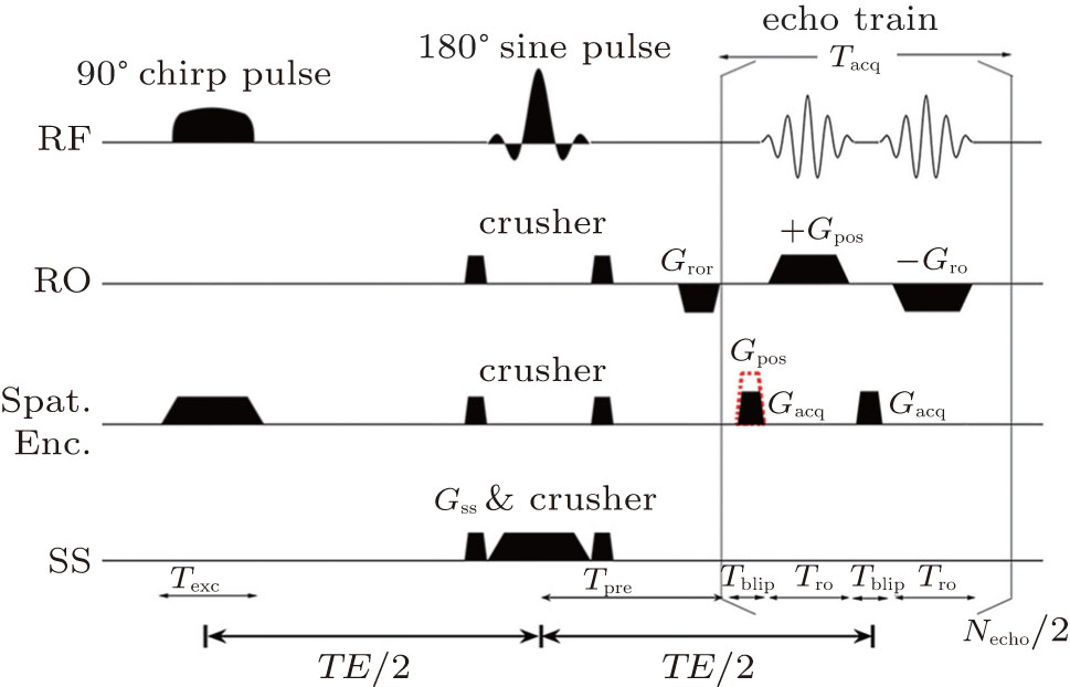
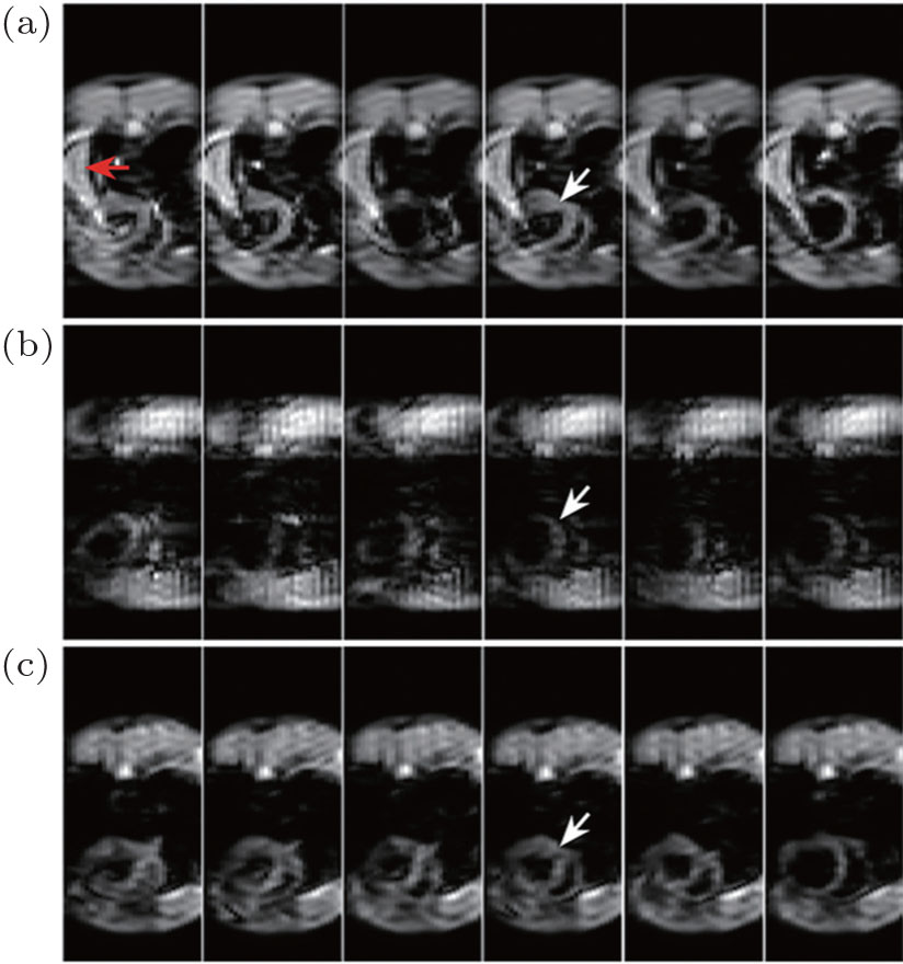
Figure 6 shows the results for the mapping of the dynamic contrast-enhanced (DCE) perfusion images of PL-DF-DOTA-Gd in rat kidney. All pulse sequences are executed with fat saturation. Figure 6(a) shows the rFOV EPI image. Figure 6(b) displays the rFOV SPEN image. When there exist severe susceptibility heterogeneities around the imaged region, e.g. the tissue-air interfaces pointed by white arrows in Figs. 6(a)– 6(c), serious geometric distortion and signal mutation appear in the rFOV EPI image (Fig. 6(a)), which may introduce errors into the mapping of DCE perfusion image. The rFOV SPEN image (Fig. 6(b)) shows better quality in the aspects of geometric shape and signal intensity uniformity. The rFOV SPEN image acquired after the steady-state magnetization condition is reached and before the contrast agent is injected, is shown in Fig. 6(d), and the one acquired near the time that the largest contrast is reached is shown in Fig. 6(e). The final image (Fig. 6(f)) is acquired after 80 min of data acquisition. The time courses of two representative pixels reflecting the renal medulla and the renal cortex are shown in Fig. 6(g). The results show the following phenomena: the deep medulla region (time course 1) displays large contrast, with contributions from the first pass of arterial perfusion as well as a slow increase in T1 weighting due to the accumulation of contrast agent in the nephrons. In the outer cortex region (time course 2), the contrast level rises rapidly due to the first pass kinetics, but then remains at a near-constant plateau as the acquisition duration is too short for the contrast agent to clear.
 | Fig. 6. DCE MR images of rat kidneys with injected contrast agent PL-DF-DOTA-Gd. (a) rFOV EPI image. (b) rFOV SPEN image. (c) Reference multi-shot gradient echo image. (d) rFOV SPEN image that is acquired after the steady-state magnetization condition has been reached and before the contrast agent is injected. (e) rFOV SPEN image acquired near the time when the largest contrast is reached. (f) Final DCE image. (g) DCE time courses of the pixels marked on the images ((d) − (f)). The time courses show the regional variation of the PL-DF-DOTA-Gd effect on the signal of medulla (1, upper) and cortex (2, bottom). |
In this study, we present a flexible rFOV imaging method and further demonstrate the superiority of the SPEN method in rFOV imaging, including high spatial resolution, high immunity to susceptibility heterogeneities and high flexibility in imaging. To evaluate this flexible rFOV imaging method, the experimental results obtained with this method are compared with those obtained with the single-shot EPI method with orthogonal RF excitation. We can find from the results that the rFOV images, including rFOV SEPN images and rFOV EPI images, show higher spatial resolutions than full FOV images. The proposed rFOV method reserves the immunity of spatiotemporal encoding to susceptibility heterogeneities. Therefore, the resulting rFOV SPEN image shows a geometric shape closer to real one than the rFOV EPI image. In addition, the rFOV image obtained with the proposed method can avoid aliasing/folding artifacts, which is a problem in EPI (e.g. the region pointed by the arrow in the left-most image in Fig. 5(a)). The proposed method also possesses the ability to perform the flexible rFOV imaging, which is demonstrated by phantom and in vivo rat head experiments, where one or two ROIs along the SPEN direction are imaged with high spatial resolution in a single shot. It would also be feasible for three-dimensional (3D) imaging. Although spatiotemporal encoding is applied in 3D imaging, the imaging time remains overlong for functional MRI or cardiac imaging. In the cases where the whole FOV scan is not necessary, the proposed rFOV SPEN imaging approach may be used to reduce the 3D imaging time. However, the experimental parameters should be chosen carefully to avoid high SAR.
It needs to be pointed out that for the proposed rFOV imaging method, the signals originating from the spins outside the ROIs might affect the signals inside the ROIs. Therefore, the rFOV images obtained with the proposed method may be disturbed by stripe artifacts. When P is reduced, this influence becomes more serious. The extent of influence is determined by the coefficient of the quadratic phase, i.e.,

which is produced by the chirp pulse together with encoding gradient. Assume that the imaged FOV Lyd and the chirp pulse are kept unchanged, then a small P will lead to a large Ly = Lyd/P and a small C2. A small C2 will lead to a wide parabolic phase which makes the interference from spins outside the ROIs serious.[22, 29] To produce a narrow parabolic phase, one can enlarge the product between the bandwidth and the duration of the chirp pulse. The interference will then be alleviated.
Another point needed to be noted is that the spatial resolution of each ROI is improved with the increase of sampled points per unit space. However, the increase of sampled points per unit space requires a longer imaging time and, consequently, the rFOV image will suffer more influence from the inhomogeneous field. Meanwhile, if the proposed rFOV imaging method is performed to obtain an ROI image with a relatively small P (e.g. P < 0.5), the strengths of encoding and decoding gradients are weak and the immunity of the method to field inhomogeneity is weakened. All these cause the rFOV SPEN image to deform along the y direction (e.g. Figs. 3(d)– 3(f) with P = 0.3) compared with the full FOV SPEN image (e.g. Fig. 3(c) with P = 1). For these reasons, the choice of P value is a tradeoff among many aspects. Empirically, the range of P value from 0.5 to 1 is optimum for the experimental samples involved in this study.
Before the proposed rFOV imaging method can be applied in clinics, the technical issue on SAR still needs to be considered. From Eq. (9), we know that the SAR is directly proportional to the bandwidth (Δ OHz) of the chirp pulse.[26, 29] Since the bandwidth (Δ OHz) of the chirp pulse used in the proposed rFOV method is the same as the one used in the fixed rFOV method, both of the rFOV SPEN methods may produce a similar SAR. Because of the large bandwidth (e.g. 64 kHz or 96 kHz used in this study), to achieve an identical flip angle, the power needed for the chirp pulse is much larger than the one required for the sinc pulse used in the rFOV EPI, thus the rFOV SPEN method will bring higher SAR. It is worth noting that the SNR of the flexible rFOV SPEN image is slightly higher than that of the rFOV EPI image (see Fig. 2). Therefore, to some extent, one can utilize a chirp pulse with a lower B1 power at the expense of a tolerable SNR reduction to reduce the SAR.
In this work, the proposed rFOV SPEN MRI method can not only achieve the desired rFOV effects including high spatial resolution and immunity to field inhomogeneity, but can also improve the SNR and can flexibly image one or more ROIs in a single shot. This might be a favorable solution to ultrafast imaging applications in cases with severe susceptibility heterogeneities, such as cardiac imaging and perfusion imaging to kidney, liver, etc. Meanwhile, it is promising in applications with separate ROIs, such as mammary and limb imaging.
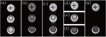
To better illustrate the principle of the flexible rFOV imaging, a series of simulations with different encoding and decoding gradients is given in Fig. A. Figures A(b)– A(e) show the region excited/encoded by the chirp pulse together with the corresponding encoding gradient. The regions circled by the dashed rectangles in Figs. A(b)– A(e) represent the ROI in each SPEN MRI experiment. The acquired SPEN data are shown in Figs. A(f)– A(i), in which the sampling trajectories are indicated by dots. The decoding/acquisition gradients along the SPEN dimension corresponding to the decoding/acquisition trajectories are shown in the bottom of Fig. A. The resulting images corresponding to Figs. A(f)– A(i) are shown in Figs. A(j)– A(m). A comparison between gradient B and gradient C indicates that the decoding/acquisition gradients used in the flexible rFOV imaging are weaker than the ones used in the fixed rFOV imaging, when the same region is imaged. The rFOV SPEN image (Fig. A(l)) obtained with the proposed method possesses a similar spatial resolution to the rFOV SPEN image (Fig. A(k)) obtained with the fixed rFOV method. Figure A(m) shows that the proposed rFOV method can image two ROIs in a single shot and the resulting SPEN image has a higher spatial resolution than the full FOV SPEN image (Fig. A(j)). It needs to be pointed out that the first blip gradient in gradient C and the fourth blip gradient in gradient D are positioning gradients, which are used to make the trajectory travel from the current ROI to the initial position of a new ROI.
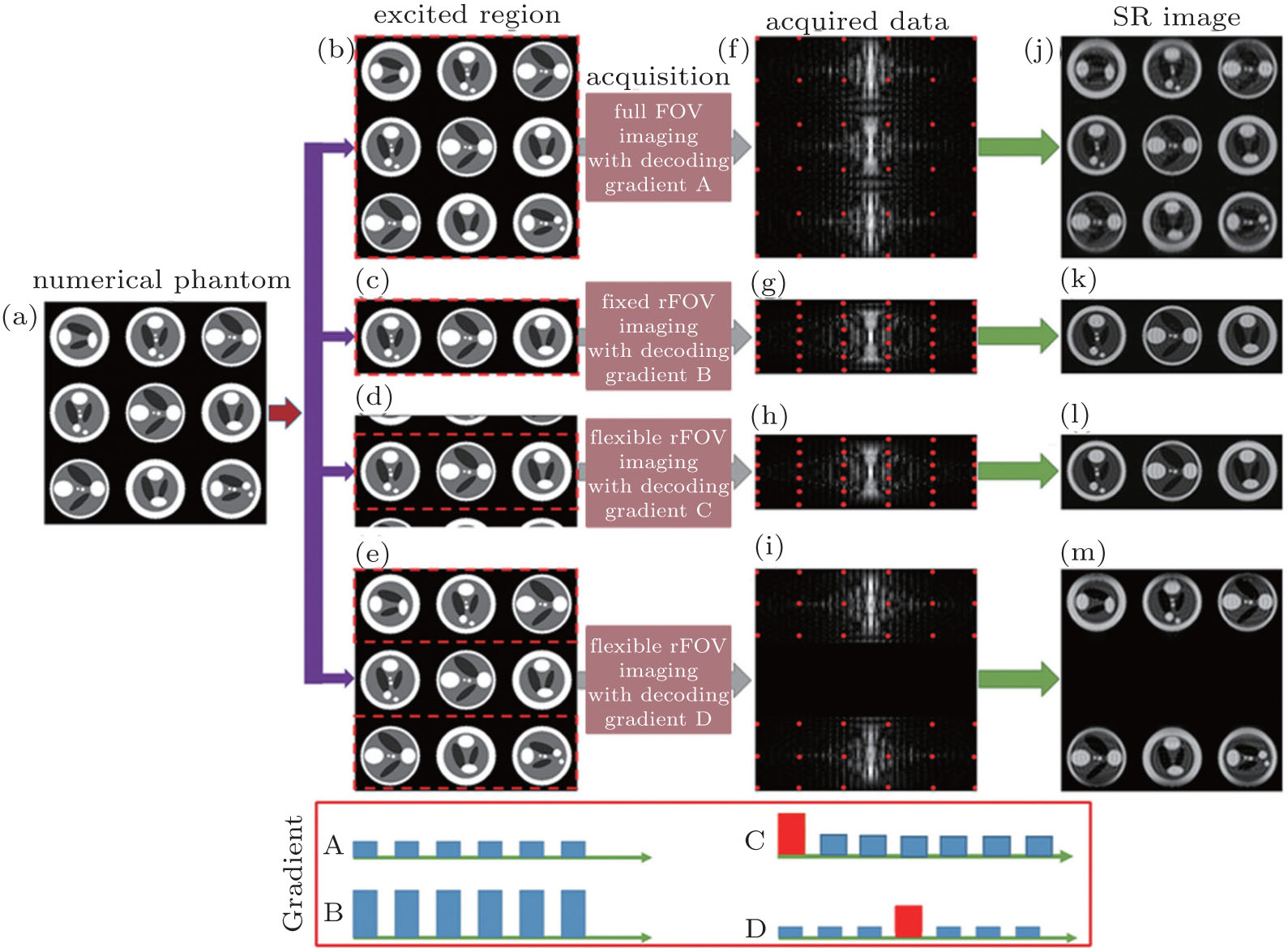 | Fig. A. Schematic diagram of the flexible rFOV imaging method. (a) Numerical phantom. (b) The excited region in full FOV SPEN MRI. (c) The excited region in fixed rFOV SPEN MRI. (d) The excited region in flexible rFOV SPEN MRI with one ROI. (e) The excited region in flexible rFOV SPEN MRI with two ROIs. (f) Full FOV SPEN data obtained with decoding gradient A. (g) Fixed rFOV SPEN data obtained with decoding B. (h) Flexible rFOV SPEN data obtained with decoding gradient C. (i) Flexible rFOV SPEN data obtained with decoding gradient D. (j)– (m) SPEN images after SR reconstruction to panels (f)– (i). Common parameters: Δ OHz = 64 kHz, Texc = 4 ms, full FOV = 6.0 cm × 6.0 cm, reduced FOV = 6.0 cm × 2.0 cm, and sampling data matrix size = 96 × 96. |
In SPEN MRI, it is convenient to obtain an original SPEN image by calculating the magnitude of the acquired time-domain signal s(ta).[24, 26, 29] The signal modulus reflects the spin density profile according to.[24, 26, 29]

Here Δ y0 denotes the pixel size and is related to the second spatial derivative of the phase arising from the initial excitation.
Although the signal modulus can reflect the spin density profile, it is blurred and its inherent spatial resolution is relatively low and cannot meet the requirements of clinical diagnosis.[24, 26, 28, 30– 32] Therefore, SR reconstruction is indispensable to improve the resolution without additional acquisition. According to the de-convolution algorithm, [30] substituting Eq. (4) into Eq. (3) and rearranging the equation, we have

In Eq. (A2), the variable of integration is y, so the constant and terms including y′ can be moved to the left side. Equation (A2) can then be expressed as follows:
The quadratic phase component has been eliminated by the transformation from s(ta) to l(y′ ), where l(y′ ) is the space-domain signal with a simple phase distribution defined as
The SR image ρ (y) can be found by solving Eq. (A3) through using the singular value decomposition (SVD) method reported previously.[31]
The discrete form of Eq. (A3) is

where L ∈ CNSR is an interpolation of l(y′ ), ρ ∈ CNSR is the SR image, and Φ ∈ C(NSR× NSR) denotes the quadratic phase modulation. ρ can be achieved by solving Eq. (A5). For the proposed flexible rFOV imaging method, according to the principle of SPEN MRI, the basic SR-reconstructed equation for the n-th ROI data can be expressed as

The SR image of n-th ROI can be found by solving Eq. (A6) through using the SR algorithm based on SVD.[31]
| 1 |
|
| 2 |
|
| 3 |
|
| 4 |
|
| 5 |
|
| 6 |
|
| 7 |
|
| 8 |
|
| 9 |
|
| 10 |
|
| 11 |
|
| 12 |
|
| 13 |
|
| 14 |
|
| 15 |
|
| 16 |
|
| 17 |
|
| 18 |
|
| 19 |
|
| 20 |
|
| 21 |
|
| 22 |
|
| 23 |
|
| 24 |
|
| 25 |
|
| 26 |
|
| 27 |
|
| 28 |
|
| 29 |
|
| 30 |
|
| 31 |
|
| 32 |
|