


Closed-form solution of mid-potential between two parallel charged plates with more extensive application
[Shang Xiang-Yu†a), b)  , Yang Chen
b) , Zhou Guo-Qinga) ]
, Yang Chen|
|


†Corresponding author. E-mail: xyshang@cumt.edu.cn
*Project supported by the National Key Basic Research Program of China (Grant No. 2012CB026103), the National Natural Science Foundation of China (Grant No. 51009136), and the Natural Science Foundation of Jiangsu Province, China (Grant No. BK2011212).
Efficient calculation of the electrostatic interactions including repulsive force between charged molecules in a biomolecule system or charged particles in a colloidal system is necessary for the molecular scale or particle scale mechanical analyses of these systems. The electrostatic repulsive force depends on the mid-plane potential between two charged particles. Previous analytical solutions of the mid-plane potential, including those based on simplified assumptions and modern mathematic methods, are reviewed. It is shown that none of these solutions applies to wide ranges of inter-particle distance from 0 to 10 and surface potential from 1 to 10. Three previous analytical solutions are chosen to develop a semi-analytical solution which is proven to have more extensive applications. Furthermore, an empirical closed-form expression of mid-plane potential is proposed based on plenty of numerical solutions. This empirical solution has extensive applications, as well as high computational efficiency.
Many biological or chemical processes involve the electrostatic interactions between biomolecules, such as proteins and nucleic acids[1– 3] or between charged particles in a colloid system. For example, electrostatic repulsive forces are known to play a crucial role in the performance of protein function.[1, 4– 8] Both electrostatic repulsive force and van der Waals force control the formation of protein complex[5, 9– 12] and the stability of the colloid system.[13, 14] Previous research has shown that the ions and potential in the electrolyte solutions in which charged colloidal particles are immersed will be redistributed, and the non-uniform potential and ions concentration will give rise to the repulsive force between particles.[13– 17] The repulsive interaction between two arbitrary inclined particles of finite length can be obtained by calculating several such interactions between two infinite parallel particles, which depend on the mid-plane potential.[18– 20] Therefore, the solution of the mid-plane potential between two infinite parallel platy particles is fundamental for research on the electrostatic interactions between irregular particles, including biomolecules.
The Poisson– Boltzmann (PB) equation is commonly used to describe the potential distribution around two charged plates.[14, 15, 21] For two separate infinite parallel plates in a symmetrical electrolyte, the dimensionless Poisson– Boltzmann equation for potential relative to bulk solution is
where ϕ = (ve/kT)ψ is the dimensionless potential, ψ is the electric potential, v is the valence of the symmetrical electrolyte, e is the elementary electric charge, k is the Boltzmann constant, T is the absolute temperature, ξ = κ y is the dimensionless distance, y is the distance from one plate surface, 
For the case of two infinite parallel plates which have the same surface potential, equation (1) can be integrated and transformed into a nonsingular nonlinear elliptic integral equation[14, 19]

where a = eϕ d, b = eϕ 0, and 
Although numerical solutions with high precision[22] can be obtained using the above numerical method, solving Eq. (2) needs numerical integration and root finding methods, both of which require many iterations and thus heavy computation cost. In a particle-scale mechanical analysis of a colloidal system which consists of thousands of colloidal particles, electrostatic repulsions between particles need to be calculated tens of thousands of times in each time step. In such a case, compared with the analytical methods which can be used to obtain the closed-form mid-plane solution, the above numerical method has very low computation efficiency. For example, for a colloidal system in which the number of particles is 1000 and 5 electrostatic repulsive forces from surrounding particles will be felt by each particle on average, 4 × 10⁸ iterations per time step are needed if the above numerical method is used and there are dozens of basic operations in each iteration. However, only 3 × 10⁵ basic operations are needed when using a typical analytical solution. In previous decades, many studies on analytical solution of PB equation were carried out.[23– 35] For two infinite parallel charged plates, Luo et al.[25, 26] obtained the analytical solutions of the PB equation on the assumption that ϕ 0 is much higher than 1 or κ h is much less than 1. Assuming that the dimensionless surface potential is very close to the mid-plane potential, Wang et al.[27] presented an analytical solution. Wang et al.[31, 32] employed the iterative method in functional theory to obtain analytical solutions of the PB equation, and stated that this approach can be used to construct an accurate and simple analytical expression at any potential. Xing[33] solved the nonlinear PB equation by introducing Weierstrass elliptic functions, and obtained the mid-plane potential analytical expressions which are applicable to small and large interparticle distance at low surface potential, and so on.
However, the above analytical solutions apply only to specific ranges of interparticle spacing and surface potential, and such a range cannot be determined quantitatively. Therefore, for two infinite parallel charged plates whose interparticle spacing or surface potential is outside of the scope of the application of the above analytical solution, it is very difficult to choose proper solution of mid-plane potential. For example, the distance between charged particles in a colloidal system subjected to external force would have so large a variation that there are many occasions where the interparticle spacing disagrees with any of the above mentioned assumptions. Therefore, it is necessary to achieve the potential solution of mid-plane between two infinite parallel charged plates, which is not only applicable to wide ranges of interparticle spacing and surface potential, but also has high computational efficiency. This paper aims to propose such a mid-plane potential solution.
The rest of this paper is organized as follows. In Section 2, the available analytical solutions of mid-plane potential between two infinite parallel charged plates are briefly introduced. Analysis with focus on the applicability of the solutions to wide ranges of interparticle spacing and surface potential is conducted. In Section 3, a semi-analytical mid-plane potential solution with extensive applicability is proposed. In Section 4, an empirical closed-form solution of mid-plane potential between two infinite parallel charged plates is put forward. This solution has extensive applicability as well as high computation efficiency. In Section 5, some conclusions are drawn from the present study.
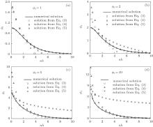
Assuming that surface potential ϕ 0 is much higher than 1, the well-known Langmuir solution[13] is obtained by neglecting the second term on the right side in Eq. (1). Utilizing a further assumption of ϕ 0 − ϕ d ≫ 1, Luo et al.[25] obtained a mid-plane potential solution in a symmetrical electrolyte as follows:

Equation (3) is only applicable for high surface potential ϕ 0 and moderate inter-plate distance κ h. Luo et al.[26] obtained a solution which is applicable to large κ h through the linear superposition of the solution of single flat double layer as follows:

However, this solution is not suitable for small κ h. Making a new assumption that (ϕ 0 – ϕ d) is close to 0, Wang et al.[27] proposed the following solution which applies to small κ h:
Figure 1 shows the numerical solution of ϕ d against κ h and the counterparts from Eqs. (3)– (5) for ϕ 0 varying between 1 and 10. Figure 1(a) shows that when ϕ 0 is 1, the solutions from Eqs. (3)– (5) are in agreement with the numerical solutions for κ h in the range from around 2 to 2.5, 3 to 10, and 0 to 2.5, respectively. However, the above scopes of the applications of solutions from Eqs. (3)– (5) change with surface potential. For example, it can be seen from Fig. 1(d) that when ϕ 0 is 10, the solutions form Eqs. (3)– (5) agree well with the numerical solutions for κ h in the range from around 1 to 4, 4 to 10, and 0 to 1. Therefore, it is difficult to choose a proper analytical solution for a given surface potential and inter-plate distance. Besides, although the solutions from Eqs. (3)– (5) almost cover the whole range of κ h from 0 to 10 as described above, there are some occasions where none of the above three analytical solutions matches with the numerical solution. For example, this is the case when ϕ 0 is 2 and κ h is around 1.8, as shown in Fig. 1(b).
2.2.1.Analytical solution based on functional theory
It has been shown in previous studies[31, 32] that the iterative method in functional theory can be used to obtain the analytical solution of Eq. (1) since the PB equation satisfies norm axioms of the functional theory and Lipschitz condition. This method needs an initial estimated solution. Although the convergence rate of the solution depends on the initial solution, the choice of the initial solution can be arbitrary. An analytical solution applicable to low potential is usually chosen to be the initial potential, which is expressed by Eq. (6). Based on Eq. (6) and the first-order iterative analytical solution (see Eq. (7)) presented by Wang et al., [32] the second-order iterative analytical solution can be obtained as Eq. (8). Its third-order iterative solution can be shown to have more than one hundred items, which will not be listed here.


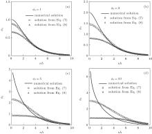
Figure 2 shows both the numerical solutions and analytical solutions from Eqs. (7) and (8) for varying ϕ 0 and κ h from 1 to 10 and to 10 respectively. Wang et al.[31, 32] stated that the iterative method only needs a first or second-order iteration to find an analytical solution without any restriction. However, it can be seen from Fig. 2(a) that when ϕ 0 is 1, the first iterative analytical solution agrees with the numerical solution for varying κ h in a wider range from around 2 to 10 than the second iterative solution. It can also be seen from Figs. 2(b)– 2(d) that the range of κ h in which the iterative analytical solution matches well with the numerical one significantly decreases with increasing ϕ 0. For example, when ϕ 0 is 5 (Fig. 2(c)), the second iterative solution matches well with the numerical solution for κ h in the range from 4.5 to 10. The error between the numerical solution and the third iterative solution is similar to those shown in Fig. 2.
 | Fig. 2. Comparisons of numerical solutions with those from functional theoretical approach for ϕ 0 = 1 (a), 2 (b), 5 (c), and 10 (d). |
2.2.2.Analytical solution based on Weierstrass elliptic functions
Using the condition of the potential symmetric with respect to the mid-plane between two infinite parallel charged plates, the integral of Eq. (1) can be obtained as follows:

Introducing a new function ℘ (ξ ) satisfying the following equation

and substituting Eq. (10) into Eq. (9) gives

where

Equation (11) is the differential equation satisfied by the Weierstrass elliptical function ℘ (ξ ; g2, g3), in which g2 and g3 are the two invariants of the function. Taking the logarithm of the both sides of Eq. (10), the dimensionless potential ϕ can be obtained as

Based on the above findings, Xing[33] obtained a series of analytical solutions of the mid-plane potential:

where γ WHP denotes the Weieristrass half period function. Solutions (13), (14), and (15) are obtained on the assumption that κ h ≪ 1 and ϕ 0 ≪ 1, κ h ≫ 1 and ϕ 0 ≪ 1, and ϕ 0 ≫ 1, respectively.
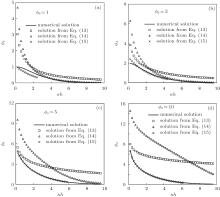
Figure 3 shows the numerical solutions as well as the analytical solutions from Eqs. (13)– (15) for ϕ 0 varying from 1 to 10 and κ h from to 10. It can be seen that equation (13) fails to match with the numerical solution, and equation (14) works well for κ h larger than 4 and 6, respectively, when ϕ 0 is 1 and 2. Equation (15) agrees well with the numerical solution when ϕ 0 is larger than 2. However, it is unsuitable for κ h smaller than 1 when ϕ 0 is 2, and does not work when ϕ 0 is 1. Furthermore, because the left side of Eq. (15) is a highly nonlinear function of mid-plane potential, equation (15) is very difficult to use for obtaining the solution of mid-plane potential for a given ϕ 0 and κ h. Besides, equation (15) is valid in a limited scope. For example, it has solutions only for κ h smaller than 5.8 and 6.4, respectively, when ϕ 0 is 5 and 10.
In summary, none of the previous analytical solutions of mid-plane potential between two infinite parallel charged plates is applicable to wide ranges of inter-plate distance from 0 to 10 and surface potential from 1 to 10. Calculating the mid-plane potential between two plates with a given arbitrary inter-plate distance and surface potential is fundamental for the mechanical analysis of colloidal system on a particle scale or that of biomolecules system on a molecular scale, so it is necessary to achieve the closed-form expression of mid-plane potential which is applicable to wide ranges of inter-plate distance and surface potential.
 | Fig. 3. Comparisons of numerical solutions with those from Weierstrass elliptic functions for ϕ 0 = 1 (a), 2 (b), 5 (c), and 10 (d). |
It has been mentioned in Section 2 that the scope of the application of the solutions as expressed in Eqs. (3)– (5) covers almost the whole range of inter-plate distance from 0 to 10 and surface potential from 1 to 10. Therefore, these three solutions are chosen to develop a new solution which has more extensive applications
Figure 1 shows that numerical curves can be divided into three parts by two points. The first point is called κ h56, at which the curve of Eq. (3) is nearest to that of Eq. (4), and the second point is called κ h57, at which the curve of Eq. (3) intersects with that of Eq. (5). When ϕ 0 is larger than 2, κ h56 is larger than κ h57. However, κ h56 is almost equal to and even smaller than κ h57 if ϕ 0 is smaller.
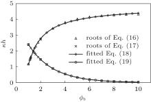
According to the above analysis, κ h56 can be seen as the root of the equation in which the first-order derivative of the difference between Eq. (4) and Eq. (3) with respect to κ h equals zero, and κ h57 can be seen as the root of the equation in which the difference between Eq. (3) and Eq. (5) equals zero. The equations, which can be used to numerically solve κ h56 and κ h57 for a given ϕ 0, are given by

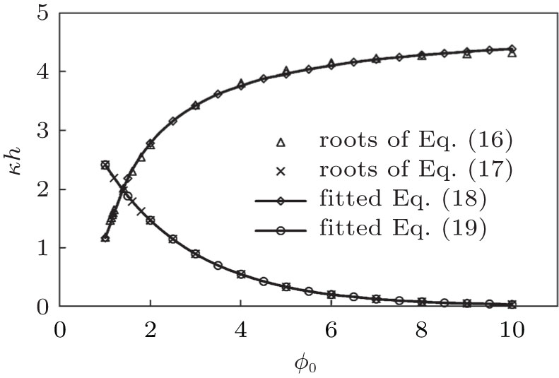
For a given ϕ 0, both of these equations can be solved by the numerical root finding method. Figure 4 shows the roots of Eqs. (16) and (17) against ϕ 0 and the corresponding fitted curves.
The equations of above mentioned fitted curves are expressed as follows:


According to Eqs. (18) and (19), κ h56 and κ h57 can be determined explicitly, and the ϕ 0 at which these two fitted curves intersect can be calculated again by numerical root finding method. It is 1.3852 and named ϕ threshold.
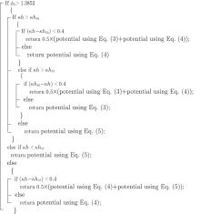
It can be observed from Fig. 1 that when ϕ 0 is larger than ϕ threshold numerical solutions corresponding to κ h < κ h57 coincide with those from Eq. (5), those corresponding to κ h56 > κ h > κ h57 coincide with those from Eq. (3), and those corresponding to κ h > κ h56 coincide with those from Eq. (4). When ϕ 0 is smaller than ϕ threshold, equation (3) is no longer suitable, and numerical solutions corresponding to κ h < κ h57 coincide with those from Eq. (5) while numerical solutions corresponding to κ h > κ h57 coincide with those from Eq. (4). Calculations suggest that none of Eqs. (3)– (5) on its own can match well with the numerical result if κ h is so close to κ h56 or κ h57 that the difference between them is smaller than 0.4. In such a case, the mean value of the solutions from Eqs. (3) and (4) when κ h is close to κ h56 or those from Eqs. (4) and (5) when κ h is close to κ h57 is closer to the corresponding numerical solution. The above analysis can be easily programmed to calculate ϕ d for given ϕ 0 and κ h. Figure 5 shows the steps of the presented solution.
 | Fig. 5. Solving steps of the proposed semi-analytical solution. |
In Fig. 6, numerical ϕ d varying with κ h is compared with those obtained from the proposed solution. It can be seen that the new solution performs well for ϕ 0 varying from 1 to 10 and κ h varying from 0 to 10. Therefore, the semi-analytical solution proposed here is applicable in a wider range than previous analytical solutions.
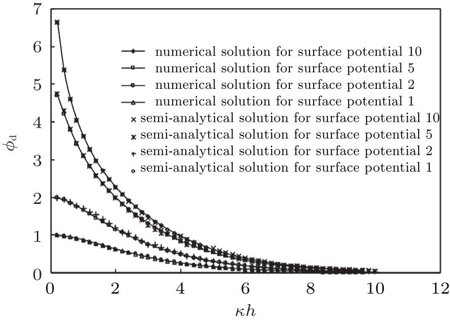 | Fig. 6. Comparisons of numerical solutions with semi-analytical ones among various surface potentials. |
As mentioned above, the semi-analytical solution is applicable to wide ranges of inter-particle spacing and surface potential. However, it involves three analytical expressions and many nested IF statements. This has a negative effect on the computational efficiency.
Based on numerical solutions of mid-plane potential between two infinite parallel charged plates whose inter-particle distance increases from 0 to 10 in steps of 0.2 and surface increases from 1 to 10 in steps of 1, an empirical mid-plane potential expression has been proposed, as follows:

in which

In the above equations, function A and relative error function B are obtained separately using the nonlinear fitting method. Figure 7 shows the empirically predicted and numerical mid-plane potential varying from 1 to 10 against dimensionless inter-particle distance varying from 0 to 10. In addition, the results for dimensionless surface potential of 1.5, 4.5, and 9.5 which are not used in the nonlinear fitting process are also shown in this figure. It can be observed that the results predicted by empirical expression Eq. (20) are in very good agreement with the numerical solutions. In addition, our calculations show that the maximum relative error is around 10%.
The presented empirical expression has more extensive applications than the analytical solutions described in Section 2. At the same time, it is more convenient and has higher computational efficiency than the semi-analytical solution described in Section 3.
 | Fig. 7. Comparisons of numerical solutions with empirical formulas at various surface potentials. |
Through the comparison of the corresponding numerical solution of mid-plane potential between two infinite parallel charged plates, the available analytical solutions are shown to be unsuitable for wide ranges of inter-plate spacing and surface potential. Based on the analysis of the selected analytical solutions, a semi-analytical solution of mid-plane potential is proposed, which has extensive applications. Furthermore, an empirical expression which can be used to estimate the mid-plane potential between two infinite parallel charged plates is put forward. This empirical solution has extensive applications as well as high computational efficiency.
| 1 |
|
| 2 |
|
| 3 |
|
| 4 |
|
| 5 |
|
| 6 |
|
| 7 |
|
| 8 |
|
| 9 |
|
| 10 |
|
| 11 |
|
| 12 |
|
| 13 |
|
| 14 |
|
| 15 |
|
| 16 |
|
| 17 |
|
| 18 |
|
| 19 |
|
| 20 |
|
| 21 |
|
| 22 |
|
| 23 |
|
| 24 |
|
| 25 |
|
| 26 |
|
| 27 |
|
| 28 |
|
| 29 |
|
| 30 |
|
| 31 |
|
| 32 |
|
| 33 |
|
| 34 |
|
| 35 |
|