Zhang Wen-Shuai, Gu Bing-Chuan, Han Xiao-Xi, Liu Jian-Dang, Ye Bang-Jiao†. Exploring positron characteristics utilizing two new positron–electron correlation schemes based on multiple electronic structure calculation methods. Chinese Physics B, 24(10): 107804
Permissions
Exploring positron characteristics utilizing two new positron–electron correlation schemes based on multiple electronic structure calculation methods
Zhang Wen-Shuaia),b), Gu Bing-Chuana),b), Han Xiao-Xia),b), Liu Jian-Danga),b), Ye Bang-Jiao†a),b)
Department of Modern Physics, University of Science and Technology of China, Hefei 230026, China
State Key Laboratory of Particle Detection and Electronics, University of Science and Technology of China, Hefei 230026, China
*Project supported by the National Natural Science Foundation of China (Grant Nos. 11175171 and 11105139).
Abstract
We make a gradient correction to a new local density approximation form of positron–electron correlation. The positron lifetimes and affinities are then probed by using these two approximation forms based on three electronic-structure calculation methods, including the full-potential linearized augmented plane wave (FLAPW) plus local orbitals approach, the atomic superposition (ATSUP) approach, and the projector augmented wave (PAW) approach. The differences between calculated lifetimes using the FLAPW and ATSUP methods are clearly interpreted in the view of positron and electron transfers. We further find that a well-implemented PAW method can give near-perfect agreement on both the positron lifetimes and affinities with the FLAPW method, and the competitiveness of the ATSUP method against the FLAPW/PAW method is reduced within the best calculations. By comparing with the experimental data, the new introduced gradient corrected correlation form is proved to be competitive for positron lifetime and affinity calculations.
In recent decades, the Positron Annihilation Spectroscopy (PAS) has become a valuable method to study the microscopic structure of solids[1– 3] and gives detailed information on the electron density and/or momentum distribution[4] in the regions scanned by positrons. An associated theory is required for a thorough understanding of the experimental results. A full two-component self-consistent scheme[5, 6] has been developed to calculate positron states in solids based on the density functional theory (DFT).[7] In particular, in bulk material where the positron is delocalized and does not affect the electron states, the full two-component scheme can be reduced without losing accuracy to the conventional scheme[5, 6] in which the electronic structure is determined by common one-component formalism. However, there are various kinds of approximations that can be adjusted within this calculation. To improve the analyses of experimental data, one should find out which approximations are more credible to produce the positron state.[8– 10] In this paper, we focus on probing the positron lifetimes and affinities by using two new positron– electron correlation schemes that are based on three electronic-structure calculation methods.
Recently, Drummond et al.[11, 12] made two calculations for a positron immersed in a homogeneous electron gas by using the Quantum Monte Carlo (QMC) method and a modified one-component DFT method, and then two forms of local density approximations (LDA) on the positron– electron correlation are derived. Kuriplach and Barbiellini[8, 9] proposed a fitted LDA form and a generalized gradient approximation (GGA) form based on previous QMC calculation, and then applied these two forms to multiple calculations for positron characteristics in a solid. However, the LDA form based on the modified one-component DFT calculation has not been studied. In this work, we make a gradient correction to the IDFTLDA form and validate these two new positron– electron correlation schemes by applying them to multiple positron lifetimes and affinities calculations.
We probe in detail the effect of different electronic-structure calculation methods on positron characteristics in a solid. These methods include the full-potential linearized augmented plane-wave (FLAPW) plus local orbitals method, [13] the projector augmented wave (PAW) method, [14] and the atomic superposition (ATSUP) method.[15] Among these methods, the FLAPW method is regarded as the most accurate method to calculate electronic structure, the ATSUP method performs with the best computational efficiency, the PAW method has greater computational efficiency and close accuracy because the FLAPW method but has not been completely tested on positron lifetimes and affinities calculations, except for some individual calculations.[16– 19] Moreover, our previous work[20] showed that the calculated lifetimes utilizing the PAW method disagree with those utilizing the FLAPW method. However, within these PAW calculations, the ionic potential was not well constructed. In this paper, we investigated the influences of the ionic pseudo-potential/full-potential and different electron– electron exchange-correlations approaches within the PAW calculations. In particular, the difference between calculated lifetimes by using the self-consistent (FLAPW) and non-self-consistent (ATSUP) methods is clearly investigated in the view of positron and electron transfers.
This paper is organized as follows. In Section 2, we give a brief and overall description of the models considered here, as well as the computational details and the analysis methods we used. In Section 3, we introduce the experimental data on positron lifetime used in this work. In Section 4, we firstly apply all approximation methods for electronic-structure and positron-state calculations to the cases of Si and Al, and give detailed analyses on the effects of these different approaches, and then assess the two new correlation schemes by using the positron lifetime/affinity data in comparison with other schemes based on different electronic-structure calculation methods.
2.Theory and methodology
2.1.Theory
In this section, we briefly introduce the calculation scheme for the positron state and various approximations investigated in this work. Firstly, we do the electronic-structure calculation without considering the perturbation by positron to obtain the ground-state electronic density ne− (r) and the Coulomb potential VCoul(r) sensed by the positron. Then, the positron density is determined by solving the Kohn– Sham equation
where Vcorr(r) is the correlation potential between electron and positron. Finally, the positron lifetime can be obtained by the inverse of the annihilation rate, which is proportional to the product of positron density and electron density accompanied by the so-called enhancement factor arising from the correlation energy between a positron and electrons.[21] The equations are written as follows:
where r0 is the classical electron radius, c is the speed of light, and γ (ne− ) is the enhancement factor of the electron density at the position r. The positron affinity can be calculated by adding electron and positron chemical potentials together:
The positron chemical potential μ + is determined by the positron ground-state energy. The electron chemical potential μ − is derived from the Fermi energy (top energy of the valence band) in the case of a metal (a semiconductor). This scheme is still accurate for a perfect lattice, as in this case the positron density is delocalized and vanishingly small at every point and thus does not affect the bulk electronic structure.[6, 21]
In our calculations, each enhancement factor is applied identically to all electrons, as suggested by Jensen.[22] These enhancement factors can be divided into two categories: the local density approximation (LDA) and the generalized gradient approximation (GGA), and they are parameterized by the following equation
here, rs is defined by rs = (3/4π ne− )1/3, ɛ is defined by ( is the local Thomas– Fermi screening length), a2, a3, a3/2, a5/2, a7/3, a8/3, and α are fitted parameters. We have investigated the five forms of the enhancement factor and the correlation potential marked by IDFTLDA, [12] fQMCLDA, [8, 9] fQMCGGA, [8, 9] PHCLDA, [23] and PHCGGA, [24] plus a new GGA form IDFTGGA introduced in this work based on the IDFTLDA scheme. The fitted parameters of these enhancement factors are listed in Table 1. The LDA forms of Vcorr corresponding to IDFTLDA, fQMCLDA, PHCLDA are given in Refs. [8], [12], and [25], respectively. Within the GGA, the corresponding correlation potential takes the form .[26, 27] The electronic density and Coulomb potential were calculated by using various methods including: a) the all-electron full potential linearized augmented plane wave plus local orbitals (FLAPW) method, [13] as implemented in Ref. [8] which is regarded as the most accurate method to calculate electronic-structure; b) the projector augmented wave (PAW) method[14] with reconstruction of all-electron and full-potential performing with greater computational efficiency and closer accuracy than the FLAPW method; and, c) the non-self-consistent atomic superposition (ATSUP) method, [15] which has the best computational efficiency.
In our calculations for the electronic structure we implemented the three methods that are mentioned above. For the FLAPW calculations, the WIEN2k code[28] was used, the PBE– GGA approach[29] was adopted for electron– electron exchange-correlations, the total number of k-points in the whole Brillouin zone (BZ) was set to 3375, and the selfconsistency was achieved up to both levels of 0.0001 Ry for total energy and 0.001 e for charge distance. For the PAW calculations, the PWSCF code within the Quantum ESPRESSO package[30] was used, the PBEsol-GGA, [31] and PZ– LDA[32] approaches were also implemented for electron– electron exchange– correlations besides the PBE– GGA approach, the PAWpseudo-potential files named PSLibrary 0.3.1 and generated by Corso (SISSA, Italy) were employed, [33] the k-points grid was automatically generated with the parameter being set at least (333) in Monkhorst– Pack scheme, the kinetic energy cut-off of more than 100 Ry (400 Ry) for the wave-functions (charge density) and the default convergence threshold of 10− 6 were adopted for self-consistency. For ATSUP calculations, the electron density and Coulomb potential for each material were simply approximated by the superposition of the electron density and Coulomb potential of neutral free atoms, [15] while the total number of the node points was set to the same as in PAW calculations. Besides, 2 × 2 × 2 supercells were used to calculate the electron structures of monovacancy in Al and Si. To obtain the positron state, the threedimensional Kohn– Sham equation, i.e. Eq. (1), was solved by the finite-difference method while the unit cell of each material was divided into about 10 mesh spaces per Bohr in each dimension. All of the important variable parameters were checked carefully to achieve that the computational precision of lifetime and affinities are in the order of 0.1 ps and 0.01 eV, respectively.
2.3.Model comparison
An appropriate criterion must be chosen to make a comparison between different models. The root-mean-squared deviation (RMSD) is the most popular and it is defined as the square root of the mean of the squared deviation between experimental and theoretical results: , here N denotes the number of experimental values. In addition, since the theoretical values can be treated to be noise-free, the simple mean-absolute-deviation (MAD) defined by is much more meaningful to quantify the overall differences between calculated results by using various models. It is obvious that the experimental data favor models producing lower values of the RMSD.
3.Experimental data
Up to five recent observed values from different literatures and groups for 21 materials were gathered to compose a reliable experimental data set. All of the experimental values for each material investigated in this work are basically collected by using the standard suggested in Ref. [57] and are listed in Table 2 with their standard deviation. Furthermore, the materials with less than five experimental measurements and/or the older experimental data were not adopted. It is reasonable to suppose that these materials have insufficient and/or unreliable experimental data that would disrupt the comparison between the models. Especially, the measurements for alkali-metals reported before 1975 are not suggested to be treated seriously.[8] The deviations of experimental results between different groups are usually much larger than the statistical errors, even when only the recent and reliable measurements are considered. That is, the systematic error is the dominant factor, so that the sole statistical error is far from enough and is not used in this work. However, the systematic error is difficult to derive from a single experimental result. In this paper, the average experimental values of each material were used to assess the positron– electron correlation models, and the systematic errors are expected to be canceled as in Ref. [57]. Because the observed values for defect state are insufficient and/or largely scattered, it is hard to make a clear discussion on the defect state by using these positron– electron correlation models in this paper. Thus, except for the detailed analyses in the cases of Si and Al based on three usually applied approaches for electronic-structure calculations, we mainly focus on testing the correlation models by using bulk materials' lifetime data and positron-affinity data. The experimental data of positron affinity are listed in Table 5.
Table 2.
Table 2.
Table 2. The experimental values of lifetime. τ exp, the related mean value and the corresponding standard deviation σ exp for each material involved in this work.
Table 2. The experimental values of lifetime. τ exp, the related mean value and the corresponding standard deviation σ exp for each material involved in this work.
4.Results and discussion
4.1.Detailed analyses in cases of Si and Al
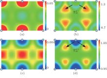
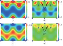
Representatively, panels (a) and (c) in Fig. 1 (Fig. 2) show, respectively, the self-consistent all-electron and positron densities on plane (110) for Al (Si) based on the FLAPW method together with the fQMCGGA form of the enhancement factor and correlation potential. It is reasonable to obtain that the panel (a) in Fig. 2 shows clear bonding states of Si while the panel (a) in Fig. 1 shows the presence of the nearly free conduction electrons in interstitial regions. To make a comparison between the FLAPW and ATSUP methods for electronic-structure calculations, we also plot the ratio of their respective all-electron and positron densities in panels (b) and (d) in Fig. (Fig. ) for Al (Si). These four ratio panels actually reflect the electron and positron transfers from densities based on the non-self-consistent free atomic calculations to that based on the exact self-consistent calculations. This confirms the fact that the positron density follows the changes of the electron density, which yield a small difference in the annihilation rate between these two calculations.[15]
Fig. 1. The self-consistent all-electron density (a) and positron density (c) (in unit of a.u., a.u. expresses atomic unit) on plane (110) for Al based on the FLAPW method and the fQMCGGA approximation. The ratios of all-electron density (b) or positron density (d) calculated by using the FLAPW method to that by using the ATSUP method.
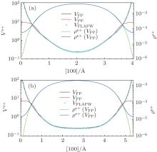
Fig. 3. The total Coulomb potential Ve+ (in unit of Ry) sensed by the positron based on the ionic pseudo-potentials (VPP) and reconstructed ionic full-potential (VFP) and the corresponding calculated positron densities ρ e+ (in unit of a.u.) along the [100] direction between two adjacent atoms for Al (a) and Si (b), respectively. To make a further comparison, the full-potentials calculated by using the FLAPW method (VFLAPW) are also plotted.
Now, taking more subtle analyses, the change of lifetime within the FLAPW calculation from that within the ATSUP calculation for Al is attributed to the competition between the following two factors: (i) the lifetime is decreased by the translations of electrons (illustrated in Fig. 1(b) as from near-nucleus regions with tiny positron densities to interstitial regions with large positron densities; and, (ii) the lifetime is increased by the translation of positron (illustrated in Fig. 1(d) as from core regions with large electron densities to interstitial regions with small electron densities. However, in the case of Si with bonding states, the change of lifetime depends conversely on the translations of electrons and positron: a) the lifetime is increased by the translations of electrons (illustrated in Fig. 2(b) as from interstitial regions with the largest positron densities to bonding regions with tiny positron densities; and, b) the lifetime is decreased by the translation of positron (illustrated in Fig. 2(d) as from the interstitial regions with tiny electron densities to bonding regions with large electron densities. Taking note of the magnitude of scale rulers, these two figures state clearly that the translations of electrons (Te− ) are dominant factors for both Al and Si. Consequently, the lifetimes within the FLAPW calculations become smaller (larger) for Al (Si). These variances are proved by calculated values of lifetimes listed in Table 3. In addition, the lifetimes of Si calculated by using three GGA forms of the enhancement factor show greater differences since the large electron-density gradient terms in bonding regions giving decreases of the enhancement factor can further weaken the effect of the translation .
We calculated the bulk lifetimes for Al and Si based on the PAW method. In Table 3, the label “ PAW” without a suffix indicates that the electron structure is calculated by using the PBE– GGA electron– electron exchange– correlations approach[32] and the positron-state is calculated by using reconstructed ionic full-potential (FP), the suffix “ – PZ” indicates that the PBE– GGA approach is replaced by the PZ– LDA approach[32] during electron-structure calculations, and the suffix “ – PP” indicates that ionic full-potential (FP) is replaced by the ionic pseudo-potential (PP) during positron-state calculations. The ionic potential together with the Hartree potential from the valence electrons compose the total Coulomb potential in Eq. (1). It can be easily found that better implementing the PAW method by using a reconstructed full-potential can give a startling agreement with the FLAPW method on the positron-lifetime calculations for Al and Si. By comparing the results of PAW and PAW– PP approaches, the PAW– PP approach leads to smaller lifetimes with the differences up to 3.8 ps and 4.3 ps for Al and Si, respectively. These decreases are caused by the fact that the softer potential within the PAW– PP approach more powerfully attracts positron into the near-nucleus regions with much larger electron densities. This statement is illustrated by the Fig. 3 showing the total Coulomb potential Ve+ sensed by the positron based on the ionic pseudo-potential (VPP) and reconstructed ionic full-potential (VFP) and the corresponding calculated positron densities ρ e+ along the [100] direction between two adjacent atoms for Al (a) and Si (b), respectively. To make a further comparison, the full-potentials calculated by using the FLAPW method (VFLAPW) are also plotted and they are found to be nearly the same as the reconstructed PAWfull-potentials. This figure indicates that a change in the ionic potential approaches (FP or PP) can lead to a change of more than one order of magnitude in the positron densities near the nuclei. It should be noted that, in the cases of PAW calculations with underestimated core/semicore electron densities in the near-nucleus regions, [58] the effect of overestimated positron densities based on the pseudo-potentials can be canceled, and then the excellent quality on the calculated positron lifetimes is able to be achieved. It is clear that the differences between the results of PAW– PZ and PAW are of the order of 0.1 ps, and therefore the effect of different electron– electron exchange– correlations schemes is small. We also calculated the lifetimes by using the PBEsol-GGA approach, [31] which is revised for solids and their surfaces, and similar differences of the order of 0.1 ps are also obtained compared with the PBE– GGA approach.
Table 3.
Table 3.
Table 3. Calculated results of positron lifetimes (in unit of ps) for Al, Si, and ideal monovacancy in Al and Si based on various methods for electronic-structure and positron-state calculations.
IDFT
IDFT
fQMC
fQMC
PHC
PHC
GGA
LDA
GGA
LDA
GGA
LDA
ATSUP
160.778
152.470
173.347
169.357
163.036
156.438
FLAPW
156.615
149.852
169.972
166.530
159.397
153.878
AI
PAW
156.649
149.898
170.016
166.584
159.432
153.925
PAW– PP
154.113
146.814
166.507
162.798
156.574
150.587
PAW– PZ
157.208
150.204
170.421
166.906
159.898
154.220
ATSUP
201.770
186.634
213.260
207.345
201.363
190.484
FLAPW
211.843
188.285
217.520
208.477
208.639
191.790
Si
PAW
211.779
188.245
217.466
208.431
208.586
191.752
PAW– PP
208.407
184.675
213.320
204.125
205.060
187.976
PAW– PZ
211.248
188.388
217.399
208.625
208.247
191.905
VAl
ATSUP
229.441
216.639
246.294
240.941
229.686
220.274
PAW
212.176
201.245
229.481
224.429
214.050
205.570
VSi
ATSUP
227.458
208.972
239.524
232.309
225.922
212.690
PAW
236.052
208.712
241.816
231.443
231.504
212.145
Table 3. Calculated results of positron lifetimes (in unit of ps) for Al, Si, and ideal monovacancy in Al and Si based on various methods for electronic-structure and positron-state calculations.
In addition, as shown in Table 3, the positron lifetimes for monovacancy in Al and Si are calculated based on the ATSUP and PAW methods for electronic-structure calculations and six correlation schemes for positron-state calculations. The ideal monovacancy structure is used in these calculations, which means that the positron is trapped into a single vacancy without considering the ionic relaxation from the ideal lattice positions. Larger differences between the results of ATSUP and PAW are found in monovacancy-state calculations compared with that in bulk-state calculations. Besides, the IDFTGGA/IDFTLDA correlation schemes produce similar lifetime values compared with the PHCGGA/PHCLDA correlation schemes and produce much smaller lifetime values compared with the fQMCGGA/fQMCLDA correlation schemes in both monovacancy-state and bulk-state calculations.
4.2.Positron lifetime calculations
In this subsection we firstly give visualized comparisons between experimental values and calculated results based on different methods for electronic-structure and positron-state calculations. Within the PAW, the positron lifetimes are all calculated by using the reconstructed full-potential and, certainly, all-electron densities from now on.
The deviations of the theoretical results from the experimental data along with the standard deviations of observed values for all materials are plotted in Fig. 4. The scattering regions of calculated results by different forms of the enhancement factor are found to be much larger in the atom systems with bonding states compared with that in pure metal systems. Besides, the deviations of the results found by using the ATSUP method from those found by using the FLAPW method are mostly larger in GGA approximations compared with those in LDA approximations. Numerically, the MADs for different forms of the enhancement factor between the calculated lifetimes by using the ATSUP method and those by using the FLAPW method are shown in Table 4. These MADs range from 1.936 ps (PHCLDA) to 5.068 ps (IDFTGGA). Moreover, the well implemented PAW method is found to be able to give nearly the same results as the FLAPW method. Numerically, the MADs between the calculated lifetimes by the PAW method and those by the FLAPW method for different forms of the enhancement factor are also shown in Table 4. These MADs range from 0.253 ps (IDFTLDA) to 0.316 ps (IDFTGGA). This near-perfect agreement between the PAW method and the FLAPW method proves that our calculations are quite credible.
Fig. 4. The deviations of the theoretical results based on various methods from the experimental values along with the standard deviation of experimental values for each material.
Table 4.
Table 4.
Table 4. The MADs between the calculated results by using the ATSUP/ PAW method and that by using the FLAPW method, and the RMSDs between the theoretical results and the experimental data .
MAD/ps
RMSD/ps
ATSUP
PAW
FLAPW
PAW
ATSUP
fQMCGGA
2.503
0.303
4.503
4.591
6.309
IDFTGGA
5.068
0.316
4.809
4.821
5.611
PHCGGA
3.667
0.287
6.148
6.013
7.672
fQMCLDA
2.184
0.290
11.36
11.19
10.35
IDFTLDA
1.966
0.253
25.19
24.99
23.88
PHCLDA
1.936
0.260
22.83
22.63
21.54
Table 4. The MADs between the calculated results by using the ATSUP/ PAW method and that by using the FLAPW method, and the RMSDs between the theoretical results and the experimental data .
Table 4 also presents the RMSDs between the theoretical results and the experimental data by using six positron– electron correlation schemes. Two interesting phenomena can be found in this table. Firstly, the RMSDs produced by the IDFTLDA scheme are always worse among the RMSDs based on three electron structure approaches, but are similar to those produced by the PHCLDA scheme. Thus, the gradient correction (IDFTGGA) to this LDA form (IDFTLDA) is needed. It is clear that the corrected IDFTGGA scheme largely improves the calculations and performs better than the PHCGGA scheme but is still worse than the fQMCGGA scheme. The fQMCGGA scheme together with the FLAPW method produced the best RMSD. This fact indicates that the quantum Monte Carlo calculation implemented in Ref. [11] is more credible than the modified one-component DFT calculation[12] on the positron– electron correlation. Secondly, compared to the RMSD produced by using the FLAPW/PAW method, the RMSD produced by using the simple ATSUP method is a little smaller based on the LDA correlation schemes but is distinctly larger based on the GGA (especially fQMCGGA) correlation schemes. This phenomenon implies that the benefit of the exact electronic-structure calculation approach (PAW/FLAPW) is swamped by the inaccurate approximation of the enhancement factor. Meanwhile, the competitiveness of the ATSUP approach against the FLAPW/PAW method is reduced based on the most accurate positron– electron correlation schemes.
4.3.Positron affinity calculations
The positron affinity A+ is an important bulk property which describes the positron energy level in a solid, and which allows us to probe the positron behavior in an inhomogeneous material. For example, the difference of the lowest positron energies between two elemental metals in contact is given by the positron affinity difference, and this determines how the positron samples behave near the interface region. Besides, if the electron work function ϕ − is known, then the positron work function ϕ + can be derived by the equation: ϕ + = − ϕ − − A+ . The crystal (e.g., W metal) with a stronger negative positron work function can emit a slow-positron to the vacuum from the surface and, therefore, can be utilized as a more efficient positron moderator for the slow-positron beam.
The theoretical and experimental positron affinities for eight common materials by using the new IDFTLDA and IDFTGGA correlation schemes are listed in Table 5. To make a comparison, the results corresponding to the PHCGGA and fQCMGGA schemes are also listed. During the electron structure calculation, the ATSUP method was not implemented because the ATSUP method is inappropriate for positron energetics calculations and gives much negative positron work functions.[15] Within PAW calculations, both PBE– GGA and PZ– LDA approaches are used for electron– electron exchange correlations. The RMSDs between theoretical and experimental positron affinities are also presented in Table 5.
Table 5.
Table 5.
Table 5. Theoretical and experimental positron affinities A+ (in unit of eV) based on four positron– electron correlation schemes and several electron structure calculation methods. The RMSDs between the theoretical and experimental positron affinities are also presented. Here, the PZ– LDA approach is labeled by PZ, and the PBE– LDA approach is labeled by PBE for short.
IDFTGGA
IDFTLDA
PHCGGA
fQMCGGA
A+
FLAPW
PAW
FLAPW
PAW
FLAPW
PAW
FLAPW
PAW
Exp
PBE
PBE
PZ
PBE
PBE
PZ
PBE
PBE
PZ
PBE
PBE
PZ
Si
– 6.481
– 6.478
– 6.683
– 6.884
– 6.881
– 7.070
– 6.728
– 6.726
– 6.926
– 6.182
– 6.179
– 6.373
– 6.2
Al
– 4.497
– 4.504
– 4.683
– 4.624
– 4.631
– 4.813
– 4.641
– 4.648
– 4.828
– 3.981
– 3.988
– 4.169
– 4.1
Fe
– 3.914
– 3.877
– 4.290
– 4.323
– 4.289
– 4.707
– 4.120
– 4.084
– 4.498
– 3.544
– 3.508
– 3.925
– 3.3
Cu
– 4.381
– 4.437
– 4.932
– 4.875
– 4.933
– 5.435
– 4.614
– 4.671
– 5.168
– 4.073
– 4.130
– 4.630
– 4.3
Nb
– 3.847
– 3.841
– 4.085
– 4.112
– 4.107
– 4.355
– 4.020
– 4.014
– 4.260
– 3.399
– 3.394
– 3.641
– 3.8
Ag
– 5.147
– 5.083
– 5.577
– 5.670
– 5.615
– 6.109
– 5.398
– 5.337
– 5.831
– 4.875
– 4.817
– 5.310
– 5.2
W
– 1.956
– 1.982
– 2.304
– 2.225
– 2.254
– 2.580
– 2.121
– 2.149
– 2.472
– 1.491
– 1.520
– 1.844
– 1.9
Pb
– 5.954
– 5.936
– 6.305
– 6.328
– 6.305
– 6.683
– 6.186
– 6.166
– 6.538
– 5.622
– 5.601
– 5.977
– 6.1
RMSD
0.285
0.283
0.546
0.570
0.566
0.899
0.431
0.427
0.740
0.314
0.314
0.272
−
Table 5. Theoretical and experimental positron affinities A+ (in unit of eV) based on four positron– electron correlation schemes and several electron structure calculation methods. The RMSDs between the theoretical and experimental positron affinities are also presented. Here, the PZ– LDA approach is labeled by PZ, and the PBE– LDA approach is labeled by PBE for short.
As in previous lifetime calculations, the calculated positron affinities found by using the FLAPW method are also nearly the same as that by using the PAWmethod. Besides, our calculated positron affinities that are found by using the fQMCGGA & PZ– LDA approaches are in excellent agreement with those reported in Ref. [8] with a MAD being 0.06 eV. Moreover, the differences between the RMSDs produced by using the PBE– GGA and PZ– LDA approaches are not negligible and the PBE– GGA approach performs much better than the PZ– LDA approach, except for the case related to fQMCGGA. In addition, the gradient correction (IDFTGGA) to the IDFTLDA form is needed to improve the performance for positron affinity calculations. Meanwhile, the IDFTGGA correlation scheme makes distinct improvement upon positron affinity calculations compared with the PHCGGA scheme, which is similar to the cases of positron lifetime calculations of bulk materials. Nevertheless, the best agreement between the calculated and experimental positron affinities is still given by the fQMCGGA & PZ– LDA approaches.
5.Conclusion
In this work, we probe the positron lifetimes and affinities utilizing two new positron– electron correlation schemes (IDFTLDA and IDFTGGA) that are based on three common electronic-structure calculation methods (ATSUP, FLAPW, and PAW). Firstly, we apply all approximation methods for electronic-structure and positron-state calculations to the cases of Si and Al, and give detailed analyses on the effects of these different approaches. In particular, the difference between calculated lifetimes by using the self-consistent (FLAPW) and non-self-consistent (ATSUP) methods is clearly investigated in the view of positron and electron transfers. The well implemented PAW method with reconstruction of all-electron and full-potential is found to be able to give near-perfect agreement with the FLAPW method, which proves that our calculations are quite credible. Meanwhile, the competitiveness of the ATSUP method against the FLAPW method is reduced by utilizing the best positron– electron correlation schemes (fQMCGGA). We then assess the two new positron– electron correlation schemes, the IDFTLDA form and the IDFTGGA form, by using a reliable experimental data on the positron lifetimes and affinities of bulk materials. The gradient correction (IDFTGGA) to the IDFTLDA form introduced in this work is necessary to promote the positron affinity and/or lifetime calculations. Moreover, the IDFTGGA performs better than the PHCGGA scheme in both positron affinity and lifetime calculations. However, the best agreement between the calculated and experimental positron lifetimes/affinities is obtained by using the fQMCGGA positron– electron correlation scheme. Nevertheless, the new introduced gradient corrected correlation form (IDFTGGA) is currently competitive for positron lifetime and affinity calculations.
Acknowledgment
We would like to thank Han Rong-Dian, Li Jun and Huang Shi-Juan for the helpful discussions. Part of the numerical calculations in this paper were completed on the supercomputing system in the Supercomputing Center of the University of Science and Technology of China.
BlahaP, SchwarzK, MadsenG K H, KvasnickaD and LuitzJ2001WIEN2k, An Augmented Plane Wave Plus Local Orbitals Program for Calculating Crystal Properties, Vienna University of Technology, Austria, 2001[Cited within:1]
PerdewJ P, RuzsinszkyA, CsonkaG I, VydrovO A, ScuseriaG E, ConstantinL A, ZhouX and BurkeK2008Phys. Rev. Lett. 100136406DOI:10.1103/PhysRevLett.100.136406[Cited within:2]
... IntroductionIn recent decades, the Positron Annihilation Spectroscopy (PAS) has become a valuable method to study the microscopic structure of solids[1#cod#x2013 ...
1
2014
0.0
0.0
1
2014
0.0
0.0
... 3] and gives detailed information on the electron density and/or momentum distribution[4] in the regions scanned by positrons ...
1
2014
0.0
0.0
... 3] and gives detailed information on the electron density and/or momentum distribution[4] in the regions scanned by positrons ...
2
1985
0.0
0.0
... A full two-component self-consistent scheme[5,6] has been developed to calculate positron states in solids based on the density functional theory (DFT) ...
... [7] In particular, in bulk material where the positron is delocalized and does not affect the electron states, the full two-component scheme can be reduced without losing accuracy to the conventional scheme[5,6] in which the electronic structure is determined by common one-component formalism ...
3
1995
0.0
0.0
... A full two-component self-consistent scheme[5,6] has been developed to calculate positron states in solids based on the density functional theory (DFT) ...
... [7] In particular, in bulk material where the positron is delocalized and does not affect the electron states, the full two-component scheme can be reduced without losing accuracy to the conventional scheme[5,6] in which the electronic structure is determined by common one-component formalism ...
... [6,21] ...
1
1965
0.0
0.0
... [7] In particular, in bulk material where the positron is delocalized and does not affect the electron states, the full two-component scheme can be reduced without losing accuracy to the conventional scheme[5,6] in which the electronic structure is determined by common one-component formalism ...
8
2014
0.0
0.0
... [8#cod#x2013 ...
... Kuriplach and Barbiellini[8,9] proposed a fitted LDA form and a generalized gradient approximation (GGA) form based on previous QMC calculation, and then applied these two forms to multiple calculations for positron characteristics in a solid ...
... We have investigated the five forms of the enhancement factor and the correlation potential marked by IDFTLDA,[12] fQMCLDA,[8,9] fQMCGGA,[8,9] PHCLDA,[23] and PHCGGA,[24] plus a new GGA form IDFTGGA introduced in this work based on the IDFTLDA scheme ...
... We have investigated the five forms of the enhancement factor and the correlation potential marked by IDFTLDA,[12] fQMCLDA,[8,9] fQMCGGA,[8,9] PHCLDA,[23] and PHCGGA,[24] plus a new GGA form IDFTGGA introduced in this work based on the IDFTLDA scheme ...
... [8], [12], and [25], respectively ...
... [8] which is regarded as the most accurate method to calculate electronic-structure ...
... [8] The deviations of experimental results between different groups are usually much larger than the statistical errors, even when only the recent and reliable measurements are considered ...
... [8] with a MAD being 0 ...
3
2014
0.0
0.0
... Kuriplach and Barbiellini[8,9] proposed a fitted LDA form and a generalized gradient approximation (GGA) form based on previous QMC calculation, and then applied these two forms to multiple calculations for positron characteristics in a solid ...
... We have investigated the five forms of the enhancement factor and the correlation potential marked by IDFTLDA,[12] fQMCLDA,[8,9] fQMCGGA,[8,9] PHCLDA,[23] and PHCGGA,[24] plus a new GGA form IDFTGGA introduced in this work based on the IDFTLDA scheme ...
... We have investigated the five forms of the enhancement factor and the correlation potential marked by IDFTLDA,[12] fQMCLDA,[8,9] fQMCGGA,[8,9] PHCLDA,[23] and PHCGGA,[24] plus a new GGA form IDFTGGA introduced in this work based on the IDFTLDA scheme ...
1
2015
0.0
0.0
... 10] In this paper, we focus on probing the positron lifetimes and affinities by using two new positron#cod#x2013 ...
2
2011
0.0
0.0
... [11,12] made two calculations for a positron immersed in a homogeneous electron gas by using the Quantum Monte Carlo (QMC) method and a modified one-component DFT method, and then two forms of local density approximations (LDA) on the positron#cod#x2013 ...
... [11] is more credible than the modified one-component DFT calculation[12] on the positron#cod#x2013 ...
4
2010
0.0
0.0
... [11,12] made two calculations for a positron immersed in a homogeneous electron gas by using the Quantum Monte Carlo (QMC) method and a modified one-component DFT method, and then two forms of local density approximations (LDA) on the positron#cod#x2013 ...
... We have investigated the five forms of the enhancement factor and the correlation potential marked by IDFTLDA,[12] fQMCLDA,[8,9] fQMCGGA,[8,9] PHCLDA,[23] and PHCGGA,[24] plus a new GGA form IDFTGGA introduced in this work based on the IDFTLDA scheme ...
... [8], [12], and [25], respectively ...
... [11] is more credible than the modified one-component DFT calculation[12] on the positron#cod#x2013 ...
2
2000
0.0
0.0
... These methods include the full-potential linearized augmented plane-wave (FLAPW) plus local orbitals method,[13] the projector augmented wave (PAW) method,[14] and the atomic superposition (ATSUP) method ...
... [26,27] The electronic density and Coulomb potential were calculated by using various methods including: a) the all-electron full potential linearized augmented plane wave plus local orbitals (FLAPW) method,[13] as implemented in Ref ...
2
1994
0.0
0.0
... These methods include the full-potential linearized augmented plane-wave (FLAPW) plus local orbitals method,[13] the projector augmented wave (PAW) method,[14] and the atomic superposition (ATSUP) method ...
... b) the projector augmented wave (PAW) method[14] with reconstruction of all-electron and full-potential performing with greater computational efficiency and closer accuracy than the FLAPW method ...
5
1983
0.0
0.0
... [15] Among these methods, the FLAPW method is regarded as the most accurate method to calculate electronic structure, the ATSUP method performs with the best computational efficiency, the PAW method has greater computational efficiency and close accuracy because the FLAPW method but has not been completely tested on positron lifetimes and affinities calculations, except for some individual calculations ...
... and, c) the non-self-consistent atomic superposition (ATSUP) method,[15] which has the best computational efficiency ...
... For ATSUP calculations, the electron density and Coulomb potential for each material were simply approximated by the superposition of the electron density and Coulomb potential of neutral free atoms,[15] while the total number of the node points was set to the same as in PAW calculations ...
... [15] ...
... [15] Within PAW calculations, both PBE#cod#x2013 ...
1
2014
0.0
0.0
... [16#cod#x2013 ...
1
2014
0.0
0.0
1
2006
0.0
0.0
1
2011
0.0
0.0
... 19] Moreover, our previous work[20] showed that the calculated lifetimes utilizing the PAW method disagree with those utilizing the FLAPW method ...
1
2014
0.0
0.0
... 19] Moreover, our previous work[20] showed that the calculated lifetimes utilizing the PAW method disagree with those utilizing the FLAPW method ...
2
1986
0.0
0.0
... [21] The equations are written as follows: ...
... [6,21] ...
1
1989
0.0
0.0
... [22] These enhancement factors can be divided into two categories: the local density approximation (LDA) and the generalized gradient approximation (GGA), and they are parameterized by the following equation ...
1
1993
0.0
0.0
... We have investigated the five forms of the enhancement factor and the correlation potential marked by IDFTLDA,[12] fQMCLDA,[8,9] fQMCGGA,[8,9] PHCLDA,[23] and PHCGGA,[24] plus a new GGA form IDFTGGA introduced in this work based on the IDFTLDA scheme ...
1
2010
0.0
0.0
... We have investigated the five forms of the enhancement factor and the correlation potential marked by IDFTLDA,[12] fQMCLDA,[8,9] fQMCGGA,[8,9] PHCLDA,[23] and PHCGGA,[24] plus a new GGA form IDFTGGA introduced in this work based on the IDFTLDA scheme ...
1
1998
0.0
0.0
... [8], [12], and [25], respectively ...
1
1995
0.0
0.0
... [26,27] The electronic density and Coulomb potential were calculated by using various methods including: a) the all-electron full potential linearized augmented plane wave plus local orbitals (FLAPW) method,[13] as implemented in Ref ...
1
1996
0.0
0.0
... [26,27] The electronic density and Coulomb potential were calculated by using various methods including: a) the all-electron full potential linearized augmented plane wave plus local orbitals (FLAPW) method,[13] as implemented in Ref ...
1
2001
0.0
0.0
... For the FLAPW calculations, the WIEN2k code[28] was used, the PBE#cod#x2013 ...
1
1996
0.0
0.0
... GGA approach[29] was adopted for electron#cod#x2013 ...
1
2009
0.0
0.0
... For the PAW calculations, the PWSCF code within the Quantum ESPRESSO package[30] was used, the PBEsol-GGA,[31] and PZ#cod#x2013 ...
2
2008
0.0
0.0
... For the PAW calculations, the PWSCF code within the Quantum ESPRESSO package[30] was used, the PBEsol-GGA,[31] and PZ#cod#x2013 ...
... We also calculated the lifetimes by using the PBEsol-GGA approach,[31] which is revised for solids and their surfaces, and similar differences of the order of 0 ...
3
1981
0.0
0.0
... LDA[32] approaches were also implemented for electron#cod#x2013 ...
... correlations approach[32] and the positron-state is calculated by using reconstructed ionic full-potential (FP), the suffix #cod#x201C ...
... LDA approach[32] during electron-structure calculations, and the suffix #cod#x201C ...
1
2014
0.0
0.0
... 1 and generated by Corso (SISSA, Italy) were employed,[33] the k-points grid was automatically generated with the parameter being set at least (333) in Monkhorst#cod#x2013 ...
1
2003
0.0
0.0
1
1989
0.0
0.0
1
1976
0.0
0.0
1
2000
0.0
0.0
1
1991
0.0
0.0
1
1997
0.0
0.0
1
1987
0.0
0.0
1
1984
0.0
0.0
1
1998
0.0
0.0
1
1998
0.0
0.0
1
1989
0.0
0.0
1
1986
0.0
0.0
1
1985
0.0
0.0
1
2004
0.0
0.0
1
2006
0.0
0.0
1
2003
0.0
0.0
1
2001
0.0
0.0
1
2003
0.0
0.0
1
1994
0.0
0.0
1
1993
0.0
0.0
1
2000
0.0
0.0
1
1986
0.0
0.0
1
1982
0.0
0.0
2
2007
0.0
0.0
... [57] and are listed in Table#cod#x00A0 ...
... [57] ...
1
2002
0.0
0.0
... It should be noted that, in the cases of PAW calculations with underestimated core/semicore electron densities in the near-nucleus regions,[58] the effect of overestimated positron densities based on the pseudo-potentials can be canceled, and then the excellent quality on the calculated positron lifetimes is able to be achieved ...
Exploring positron characteristics utilizing two new positron–electron correlation schemes based on multiple electronic structure calculation methods
[Zhang Wen-Shuaia),b), Gu Bing-Chuana),b), Han Xiao-Xia),b), Liu Jian-Danga),b), Ye Bang-Jiao†a),b)]


 ]
]