Effect of microwave frequency on plasma formation in air breakdown at atmospheric pressure
[Zhao Peng-Cheng† , Guo Li-Xin, Li Hui-Min]
, Guo Li-Xin, Li Hui-Min]
|
|


†Corresponding author. E-mail: pczhao@xidian.edu.cn
*Project supported by the Fundamental Research Funds for the Central Universities, China and the National Natural Science Foundation of China (Grant No. 61501358).
Microwave breakdown at atmospheric pressure causes the formation of a discrete plasma structure. The one-dimensional fluid model coupling Maxwell equations with plasma fluid equations is used to study the effect of the microwave frequency on the formation of air plasma. Simulation results show that, the filamentary plasma array propagating toward the microwave source is formed at different microwave frequencies. As the microwave frequency decreases, the ratio of the distance between two adjacent plasma filaments to the corresponding wavelength remains almost unchanged (on the order of 1/4), while the plasma front propagates more slowly due to the increase in the formation time of the new plasma filament.
In recent years, the filamentary plasma array formation during the gas breakdown at atmospheric pressure caused by the high-power microwave with the frequency of 110 GHz has been extensively studied, [1– 8] since its applications involve plasma processing, directed energy weapons, ionospheric modification, and so on. Hidaka et al. observed that the array including several plasma filaments and propagating toward the microwave source is formed at and around atmospheric pressure.[1, 2] Experiments performed by Cook et al. showed that decreasing the gas pressure leads to the transition of plasma structure from a filamentary plasma array to diffusion plasma.[3] Nam et al., [4] Boeuf et al., [5– 7] and Zhou et al.[8] have well explained these experimental results by using the fluid models, respectively. In fact, the discrete plasma structure at 110 GHz is similar to those at lower microwave frequencies in Refs. [9] and [10]. However, we know little about the effect of the microwave frequency on plasma formation at atmospheric pressure.
In this paper, we use the one-dimensional (1D) fluid model[7, 11– 13] to simulate the interaction of the high-power microwave with the weak ionized plasma at different microwave frequencies. Although the one-dimensional (2D) model cannot capture the two-dimensional nature of filaments observed in experiments, [1– 3, 9, 10] it can explain the difference in the plasma formation caused by the microwave frequency. The reasonable electron diffusion coefficient[5] that considers the transition from the free diffusion in the plasma front to the ambipolar diffusion coefficient in the plasma bulk is introduced into the current model. These frequency parameters such as the ionization frequency are obtained from empirical scaling laws.[14]
We use the 1D fluid model to describe the air breakdown caused by the plane wave. The microwave with polarization direction parallel to the x axis propagates in the positive z-axis direction. In this case, the basic equations for the model can be expressed as[7]


where Ex is the electric field component along the x axis, Hy is the magnetic component along the y axis, e and me denote the charge and mass of electron, respectively, ɛ 0 and μ 0 are the permittivity and permeability of free space, respectively, Deff is the electron diffusion coefficient, ν i, ν a, and ν m are the ionization frequency, attachment frequency, and collision frequency, respectively, Ne denotes the free electron density, and vx is the electron velocity along the x axis.
These frequency parameters in Eqs. (3) and (4) can be obtained from empirical scaling laws[14]


In Eqs. (5)– (7), the effective electric field

the critical field Ec = 32p whose unit is V/cm and the pressure p is measured in Torr (1 Torr = 1.33322× 10² Pa).
The effective electron diffusion coefficient Deff that is assumed to be spatially uniform is written as[5]


where α is the local Maxwell relaxation time, and μ e and μ i are the electron mobility and ion mobility, respectively. From Eqs. (8)– (11), we can see clearly that α controls the transition from the free diffusion in the plasma front (α ≈ or > 1) to the ambipolar diffusion coefficient in the plasma bulk ( α ≪ 1).
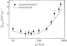
The finite-difference time-domain numerical scheme proposed in Ref. [6] is employed to solve Eqs. (1)– (4) numerically. The simulation domain is 0 < z < 3 λ , where λ represents the wavelength. The initial values of variables without Ne, i.e., Ex, Hy, and vx, are taken to be zero. In order to validate the fluid model with these coefficients shown in Eqs. (5)– (11), we simulate the breakdown thresholds of a microwave pulse with the frequency of 110 GHz and the width of 2.5 μ s over a wide range of air pressures and compare them with the experimental data, [3] as shown in Fig. 1. The reason for choosing such a frequency is because the corresponding experiment is available in previous studies. The breakdown threshold is defined as the root-mean-square (rms) electric field of the microwave pulse when the electron density has reached 108 times the initial level during a period of the pulse width.[4, 12] We see from Fig. 1 that the simulated breakdown thresholds are very well matched with the experimental data. It should also be pointed out that the fluctuations in the experimental data are caused by the seed electron.[15]
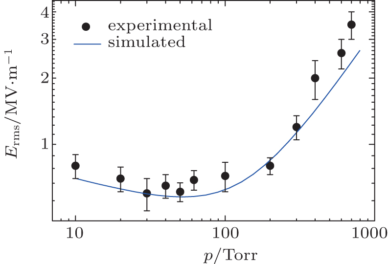 | Fig. 1. Comparison between simulated breakdown thresholds and experimental data while the frequency and width of microwave pulse are 110 GHz and 2.5 μ s, respectively. |
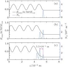
We assume that the initial (seed) electrons exit only around z = 2λ and their density profile is similar to a Gaussian shape with a standard deviation of 50 μ m and a maximum value of 1 × 10¹⁵ m− 3. The background gas is air and its pressure is taken to be 760 Torr. The microwave source is added at z = 0. The amplitude of the incident microwave Ei, m = 6 MV/m, and its frequency f is taken to be 110, 55, and 11 GHz, respectively. Figures 2– 4 show the spatial distributions of the root-mean-square electric field normalized by 
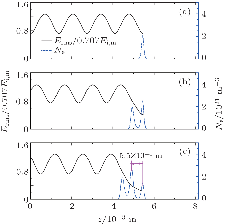 | Fig. 2. Spatial distributions of root-mean-square electric field normalized by  |
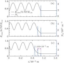
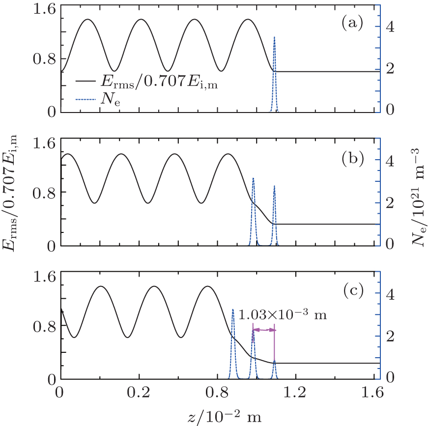 | Fig. 3. Spatial distributions of root-mean-square electric field normalized by |
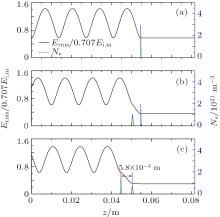
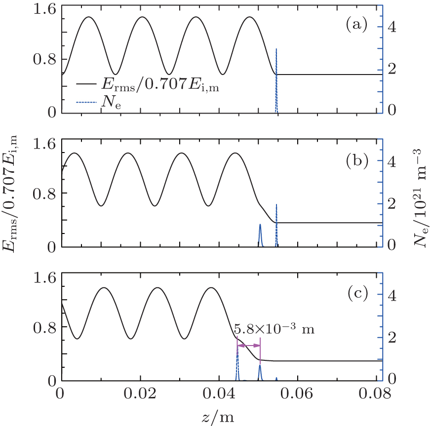 | Fig. 4. Spatial distributions of root-mean-square electric field normalized by |
We see from Fig. 2(a) that, at f = 110 GHz, the density and thickness of the plasma at t = 30 ns become large compared to their initial values. The plasma front reflects the microwave and then the standing wave appears. At t = 40 ns, the new plasma filament has been formed around the location, where the electric field was close to the maxima, as shown in Fig. 2(b). This is due to the combination of diffusion and ionization in the enhanced field. The density of the new filament grows till the electric field inside the filament becomes smaller than the critical field, at which the ionization frequency equals the electron loss frequency. The processes similar to those shown in Figs. 2(a) and 2(b) occur continually with time. As a result, the new plasma filament appears again after a longer time, as shown in Fig. 2(c). The electric field inside the downstream plasma filaments is much lower than the critical field, since it is reflected and absorbed by the plasma array. In this case, the electron loss processes are dominant over the ionization process, and the density of the downstream plasma filament decays with time, as shown in Fig. 2(c). The results above are in excellent agreement with the experimental phenomenon[1– 3] and other simulations.[4– 8]
Figures 3 and 4 show that the plasma structures similar to the case of f = 110 GHz are formed at lower microwave frequencies. The maximum density of the plasma filament at the three different microwave frequencies is on the order of 1021 m− 3. Although the distance between the two adjacent plasma filaments becomes larger at a lower microwave frequency, the ratio of the distance to the corresponding wavelength shows a little change, which is approximately equal to 0.8/4. The experimental value of the ratio is about 1/4. The little difference can refer to the explanation presented by Zhou et al.[8] From Figs. 4, we can speculate that the array including several plasma filaments seems to disappear at f = 11 GHz. However, the experimental results showed that the array including several plasma filaments appears clearly around this microwave frequency.[9, 10] The disparity between simulated and experimental results can be explained by the fact that the electron loss frequency involving the attachment and electron diffusion is somewhat overestimated, and the sustaining time of the downstream plasma filament is shortened obviously.
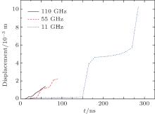
Figure 5 shows the displacement of the plasma front (edge of the first filament on the left in Figs. 2– 4) relative to its initial location z ∼ 2λ as a function of time for different microwave frequencies. The position of the plasma front is determined by following a particular density level on the z axis. According to Ref. [7], the level is taken as 1017 m− 3. It can be seen from Fig. 5 that the speed of the front propagation is not constant. This is because the newly formed filament takes some time to reach a significant density level before it starts reflecting the microwave and propagates forward. As the microwave frequency decreases, the formation time of the filament becomes longer. As a result, the plasma front propagates more slowly at the lower microwave frequency.
 | Fig. 5. The displacement of the plasma front relative to its initial location z ∼ 2λ versus time for different microwave frequencies. |
We have investigated the effect of the microwave frequency on the plasma formation in air breakdown at atmospheric pressure by using the fluid model. The reasonable electron diffusion coefficient and empirical scaling laws for frequency parameters were adopted in the fluid model. We simulated the breakdown thresholds of a microwave pulse in air which are very well matched with the experimental data. It was found that similar arrays including several plasma filaments and propagating toward the source are formed at different microwave frequencies. The ratio of the distance between two adjacent plasma filaments to the corresponding wavelength is on the order of 1/4, and the maximum plasma density is on the order of 10− 21 m− 3. As the microwave frequency decreases, the plasma front propagates more slowly. This can be explained by the fact that decreasing the microwave frequency leads to the increase in the formation time of the new plasma filament.
| 1 |
|
| 2 |
|
| 3 |
|
| 4 |
|
| 5 |
|
| 6 |
|
| 7 |
|
| 8 |
|
| 9 |
|
| 10 |
|
| 11 |
|
| 12 |
|
| 13 |
|
| 14 |
|
| 15 |
|