The high-order nonlinear Schrö dinger equation with a trapped term (HNLSET)^[1] is

where , m is a positive integer, α is a constant, ħ (| u| ²) is a bounded real differentiable function of | u(x, t)| ², and g(x) is a real-valued bounded function. The potential term g(x) is to localize the wave around the origin. The equation has been used to describe many physical phenomena and widely applied to many important physical contexts, such as fluid dynamics, nonlinear optics, quantum physics, plasma physics, and Bose– Einstein condensates. With initial and periodic boundary conditions u(x, 0) = u₀(x), x ∈ [a, b], , t ∈ [0, T], s = 1, 2, … , m − 1. The HNLSET has charge conservation law

and energy conservation law

There have been some works for the HNLSET in special cases. For m = 1, g(x) = 0, and ħ (| u| ²) = | u| ⁴, the equation will be nonlinear Schrö dinger (NLS) equation, which has been solved by various methods.^{[1– 5]} For m = 1 and ħ (| u| ²) = | u| ⁴, the equation is called trapped NLS equation. Pé rez-Garcí a and Liu^[6] proposed several numerical methods for the equation with g(x) = − x²/2 and Wang^[7] suggested the split-step finite difference method. In Ref. [8], Dehghan and Taleei proposed a time– space method for the numerical solution of the trapped NLS equation. In Ref. [9], Hong and Kong discussed some multi-symplectic algorithms for the HNLSET with ħ (| u| ²) = 3| u| ⁴ and g(x) = − 150sin²x.

For the HNLSET (1), some authors also have done some works. Chao^[10] proposed a charge and energy-preserving finite difference scheme. In Ref. [11], Zeng derived an explicit and conditionally stable leap– frog difference scheme. In Ref. [12], Kong et al. proposed a symplectic scheme for the problem. Although there have been some methods for the HNLSET (1), most of them are not energy-preserving. Spectral and pseudospectral methods have been very popular in recent decades because of their convergence accuracy in solving smooth problem, especially with the advent of the fast Fourier transform. Thus, the problem now is whether we can design a stable and efficient Fourier pseudospectral method for the HNLSET (1) as well as preserving the two conserved quantities (2) and (3).

The arrangement of this paper is as follows. In Section 2, we construct a Fourier pseudospectral method for the HNLSET (1). Then, we analyze the charge and energy conservative properties. Some numerical experiments are presented in Section 3. We finish the paper with a summary in the last section.

In order to derive the method conveniently, we introduce some notations: x_j = a + jh, t_n = nτ , j = 0, 1, 2, … , J; n = 0, 1, 2, … , where J is an even integer, h = (b − a)/J and τ are spatial length and temporal step span. Let be the approximation of and . Denote the finite difference and average operators as and . Define vector inner product and vector L₂-norm as and .

As we know, the best merit of the spectral and pseudospectral methods is their rapid convergence accuracy in solving smooth problems. We approximate u(x, t) by , where and g_k(x) are interpolation basis functions. In practice, there are many feasible choices of basis functions, such as Fourier trigonometric polynomials, Chebyshev polynomials, Legendre polynomials, and so on. For a practical problem, we should choose suitable basis functions. Because of the periodic boundary conditions, we choose

where μ = 2π /(b − a). The first-order differential operator ∂ _x yields the Fourier spectral differentiation matrix D₁ ∈ ℝ ^{J× J} with entries

j, k = 0, 1, … , J − 1. It is worth noting that D₁ is skew-symmetric. Generally, the Fourier spectral differentiation matrix for ∂ _xx is D₂ (see Ref. [13]). In Refs. [9], [13]– [18], the authors used and to approximate differential derivatives ∂ _xxu(x, t) and . Actually, we can use to approximate . By using the discrete Fourier transform, we have the following relationships

where p is a positive integer, is the matrix of discrete Fourier transform coefficients with entries given by , ω = e^{− i2π /J}, and Λ is a diagonal matrix whose (non-zero) entries are the scaled wave-numbers

Applying the midpoint rule with respect to time and the Fourier pseudospectral method with respect to space in HNLSET (1), we have a scheme

where g_j denotes the value of g(x_j). In order to analyze its conservative properties conveniently, we rewrite the scheme (4) into a vector form

where g = (g₀, g₁, … , g_{J − 1})^T and ‘ · ’ represents point multiplication between vectors, i.e., u· v = (u₀v₀, u₁v₁, … , u_{J − 1}v_{J − 1})^T. Next, we will present some conservative properties of the method (5).

Remark 1 As usual, should be approximated by , but not by . Here, we should point out that is not equal to D_2m. The reason for the choice is as follows: First, the authors^{[13– 15, 18]} have used to approximate successfully; Second, the best merit of the choice is that we can obtain a discrete energy conservation law consisted with Eq. (3).

Theorem 1 With the initial and periodic boundary conditions, the method (5) preserves the charge conservation law exactly, that is

Proof Taking the inner product of Eq. (5) with u^{n + 1} + uⁿ yields

The first term becomes

where stands for the imaginary part. The second term

is real. The last term is also real. Thus, the imaginary part of Eq. (7) implies the discrete charge conservation law (6).   ◻

Remark 2 The discrete charge conservation law is unitary. Thus, the scheme (5) is unconditionally stable with respect to the initial values.

Theorem 2 For the periodic boundary conditions, the scheme (5) satisfies the implicit discrete energy conservation law

Proof Computing the inner product of scheme (5) with u^{n + 1} − uⁿ yields

The first term is a pure imaginary one. The second term becomes

One derives immediately from the third term that

The last term

Therefore, taking the real part of Eq. (9), we complete the proof.   ◻

Remark 3 Theorem 2 implies that the scheme (5) does not explicitly conserve the energy conservation law over time in the general case. The reason is that the terms

cannot be vanished. However, for some special case of ħ (| u| ²), we will have an explicit energy conservation law.

Corollary 1 If ħ (| u| ²) = ρ , where ρ is a given constant, then we have explicit discrete energy conservation law .

Corollary 2 For the case of ħ (| u| ²) = ρ | u| ², where ρ is a given constant, the following explicit discrete energy conservation law is held .

Corollary 3 If ħ (| u| ²) = ρ | u| ⁴, where ρ is a given constant, the scheme (5) possesses explicit discrete energy conservation law

where

In this section, we will test the numerical accuracy and preservation of the proposed method (5) for the HNLSET (1). In the following computations, the accuracies of the numerical solutions are calculated by

and , and the errors in charge and energy invariants are scaled by and .

3.1.Linear Schrö dinger equation

Consider the linear test problem , , , s = 0, 1, 2, ..., m − 1. The theoretical solution of the problem is u(x, t) = exp(i (t − π /4))sin x. According to Theorem 1 and Corollary 1, the present method preserves the discrete charge and energy invariants exactly. Here, we solve the problem for m = 1, 2, 3 with initial condition u₀(x) = u(x, 0) and temporal step τ = 0.0001 up to T = 2. Kong et al.^[12] investigated the problem by two symplectic schemes, which are respectively called M2L1 and M2L2. Computational results are displayed in Table 1. It is clear that the present scheme (5) provides accurate solution and conserves charge and energy invariants to machine accuracy. Further, one can see the performance of the present method is much better than that of M2L1 and M2L2.

Table 1.

Table 1.

Table 1. The errors in solution, charge and energy at T = 2. m Method h e2 e∞ 1 Present π /20 2.954× 10− 9 1.666× 10− 9 1.199× 10− 14 1.376× 10− 14 π /40 2.953× 10− 9 1.666× 10− 9 6.217× 10− 15 2.664× 10− 15 M2L1 π /20 2.886× 10− 3 4.109× 10− 3 1.806× 10− 12 1.148× 10− 11 π /40 5.106× 10− 4 1.028× 10− 3 2.149× 10− 13 2.707× 10− 12 M2L2 π /20 9.484× 10− 6 1.350× 10− 5 2.358× 10− 11 2.929× 10− 13 π /40 4.206× 10− 7 8.467× 10− 7 1.701× 10− 11 1.992× 10− 13 2 Present π /20 2.955× 10− 9 1.670× 10− 9 1.954× 10− 14 1.687× 10− 14 π /40 2.507× 10− 9 1.458× 10− 9 8.881× 10− 16 1.687× 10− 14 M2L1 π /20 5.767× 10− 3 8.029× 10− 3 3.093× 10− 12 2.144× 10− 11 π /40 1.020× 10− 3 2.055× 10− 3 3.438× 10− 12 2.145× 10− 10 M2L2 π /20 2.486× 10− 5 3.539× 10− 3 1.349× 10− 11 8.896× 10− 11 π /40 1.102× 10− 6 2.219× 10− 6 1.148× 10− 12 4.708× 10− 10 3 Present π /20 7.781× 10− 9 4.639× 10− 9 9.648× 10− 12 9.550× 10− 12 π /40 1.194× 10− 6 1.067× 10− 6 7.662× 10− 11 7.763× 10− 11 M2L1 π /20 8.641× 10− 3 1.230× 10− 2 8.807× 10− 11 2.035× 10− 9 π /40 1.530× 10− 3 3.082× 10− 3 1.893× 10− 9 1.739× 10− 7 M2L2 π /20 4.610× 10− 5 6.562× 10− 5 2.595× 10− 11 3.875× 10− 9 π /40 2.057× 10− 6 4.412× 10− 6 5.847× 10− 10 4.041× 10− 7

Table 1. The errors in solution, charge and energy at T = 2.

3.2.Nonlinear Schrö dinger equation

In order to get insight into the performance of the method for the nonlinear problem, we consider the NLS equation iu_t + u_xx + 2| u| ²u = 0.

Example 1 (soliton solution) NLS equation admits the exact soliton solution

We take u₀(x) = u(x, 0, 2, 0), − 10 ≤ x ≤ 10 as the initial condition. The computational parameters are τ = 0.01 and J = 200. The numerical results are listed in Table 2. One can see the errors in solutions are satisfactory and the errors in charge and energy invariants are within the roundoff error of the machine.

Table 2.

Table 2.

Table 2. The errors in solution, charge, and energy for NLS equation. Time e∞ e2 T = 10 3.350× 10− 4 5.442× 10− 4 2.264× 10− 14 3.108× 10− 15 T = 20 6.703× 10− 4 1.091× 10− 3 4.218× 10− 15 3.108× 10− 15 T = 30 9.941× 10− 4 1.631× 10− 3 2.420× 10− 14 3.552× 10− 15 T = 40 1.631× 10− 3 2.177× 10− 3 3.108× 10− 15 2.664× 10− 15

Table 2. The errors in solution, charge, and energy for NLS equation.

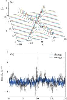
Example 2 (solitons collision) We consider initial condition u₀(x) = u(x, 0, 2, − 20) + u(x, 0, − 2, 20) over the region − 40 ≤ x ≤ 40. The simulations are done with τ = 0.01 and J = 200 up to T = 20. The interaction of the two solitons is illustrated with Fig. 1(a). The two solitons move in opposite directions and merge into a large wave at T = 10. After the interaction, both of them bound back along their original paths with original shapes and velocities. Figure 1(b) shows the errors in charge and energy. It is clear that the two invariants are conserved exactly.

Fig. 1.

	Figure Option ViewDownloadNew Window
	Fig. 1. (a) Two solitons’ collision for NLS equation; (b) the errors in charge and energy invariants.

3.3.Second-order NLS equation with a trapped term

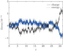
We consider equation iu_t + u_xx − cos²xu − | u| ²u = 0 with initial condition u₀(x) = sinx, x ∈ [0, 2π ]. Wang^[7] studied this problem by using the split-step finite difference (SSFD) method. The equation has the exact solution u(x, t) = sinx exp(− i3t/2). We compute the problem with τ = 0.01, J = 128 up to T = 32. The maximum errors at various times are shown in Table 3. We see that the present method provides a more accurate solution than SSFD. The residuals of charge and energy are displayed in Fig. 2.

Table 3.

Table 3.

Table 3. The maximum errors in solution at various times. Method T = 4 T = 12 T = 20 T = 28 T = 32 Pesent 1.125× 10− 4 3.374× 10− 4 5.624× 10− 4 7.874× 10− 4 8.999× 10− 4 SSFD[7] 4.0574-4 1.217× 10− 3 2.209× 10− 3 2.840× 10− 3 3.246× 10− 3

Table 3. The maximum errors in solution at various times.

Fig. 2.

	Figure Option ViewDownloadNew Window
	Fig. 2. The errors in charge and energy invariants for NLS with a trapped term.

3.4.Fourth-order NLS with a trapped term

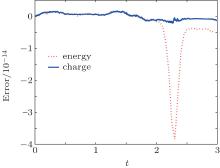
We study the the following fourth-order NLS equation with a sine-trapped term and 2π -periodic initial value problem iu_t + u_xxxx − 150(sinx)²u + 6 | u| ²u = 0, , u(x, t) = u(x + 2π , t) = 0 u_xx(x, t) = u_xx(x + 2π , t) = 0. The problem admits a theoretical solution u(x, t) = 5exp(i(t + π /4))sin x. In the following tests, we will compare the numerical behaviors of the present method (5) with those of schemes E-P, ^[10] L-F, ^[11] M2L1, and M2L2.^[12] Table 4 lists the computational results with various mesh grid divisions at T = 1. The results in the table reveal that the present scheme provides a more accurate solution than other methods. Next, we study the performance of the scheme in preserving invariants. We simulate the problem with the computational parameters τ = 5 × 10^{− 4} and J = 80 up to T = 3. From Fig. 3, we see the errors in charge and energy are smaller than 10^{− 10}. They oscillate near zero and do not exhibit marked growth against time. From the literature, ^[12] one sees the errors in charge and energy obtained by E-P, L-P, M2L1, and M2L2 schemes increase rapidly after T = 2.5. Thus, the present method is much more efficient than those methods.

Table 4.

Table 4.

Table 4. The errors in solution T = 1. τ h Method e2 e∞ 4× 10− 6 π /20 L-P 1.447× 10− 2 2.052× 10− 2 1× 10− 3 π /20 E-P 1.441× 10− 2 2.052× 10− 2 1× 10− 3 π /20 M2L1 1.450× 10− 2 2.064× 10− 2 1× 10− 3 π /20 M2L2 1.501× 10− 4 2.141× 10− 4 1× 10− 3 π /20 present 7.386× 10− 7 4.202× 10− 7 2× 10− 6 π /40 L-P 2.552× 10− 3 5.138× 10− 3 5× 10− 6 π /40 E-P 2.552× 10− 3 5.138× 10− 3 5× 10− 4 π /40 M2L1 2.567× 10− 3 5.169× 10− 3 5× 10− 4 π /40 M2L2 1.832× 10− 5 3.697× 10− 5 5× 10− 4 π /40 present 7.689× 10− 7 4.441× 10− 7

Table 4. The errors in solution T = 1.

Fig. 3.

	Figure Option ViewDownloadNew Window
	Fig. 3. The errors in invariants for the fourth-order NLS equation with a trapped term.

For the HNLSET (1) with periodic boundary conditions, we apply the Fourier pseudospectral method with respect to space and the midpoint rule with respect to time, and then derive a new scheme. We prove the method conserves the charge and energy conservation laws exactly. Various numerical experiments are implemented to exhibit the performance of the method. Numerical results verify the proposed scheme is charge- and energy-conserved, and also reveal it is more efficient than many existing methods.

The present method can also be applied to two- or three-dimensional problems. To illustrate this, we consider two-dimensional NLS equation

on spatial domain [x_L, x_R] × [y_L, y_R] with periodic boundary conditions. For simplicity, let h_x = (x_R − x_L)/J and h_y = (y_R − y_L)/J. Since the matrix is symmetric, applying the midpoint rule with respect to time and the Fourier pseudospectral method to Eq. (10) gives a matrix equation

where the entries of the matrix Uⁿ satisfy [Uⁿ]_{j, k} = u(x_j, y_k, t_n). Because of , multiplying Eq. (11) from the left by and from the right by , we have

where and the matrix

The system of the nonlinear equations can be solved by a simple iterative method, i.e.,

where q means the iterative step. Further, using the relation yields the solution matrix U. The scheme (11) is also charge- and energy-preserved. Because of the limitation in length of the journal, the numerical analysis and numerical experiments will be presented in another paper.