


Analysis of elastoplasticity problems using an improved complex variable element-free Galerkin method
[Cheng Yu-Min†a)  , Liu Chao
a) , Bai Fu-Nonga) , Peng Miao-Juanb) ]
, Liu Chao|
|


†Corresponding author. E-mail: ymcheng@shu.edu.cn
*Project supported by the National Natural Science Foundation of China (Grant Nos. 11171208 and U1433104).
In this paper, based on the conjugate of the complex basis function, a new complex variable moving least-squares approximation is discussed. Then using the new approximation to obtain the shape function, an improved complex variable element-free Galerkin (ICVEFG) method is presented for two-dimensional (2D) elastoplasticity problems. Compared with the previous complex variable moving least-squares approximation, the new approximation has greater computational precision and efficiency. Using the penalty method to apply the essential boundary conditions, and using the constrained Galerkin weak form of 2D elastoplasticity to obtain the system equations, we obtain the corresponding formulae of the ICVEFG method for 2D elastoplasticity. Three selected numerical examples are presented using the ICVEFG method to show that the ICVEFG method has the advantages such as greater precision and computational efficiency over the conventional meshless methods.
The meshless method is a numerical method proposed in the middle of the 1990s. Compared with the conventional numerical methods, the meshless method does not discretize the solution domain into a mesh, but only requires the information about nodes in the domain. The meshless method can be used to solve some complicated problems which cannot be solved well with traditional numerical methods, such as the finite element method and the boundary element method.[1– 3]
The element-free Galerkin (EFG) method[1] is one of the most important meshless methods. The moving least-squares (MLS) approximation[4] is used in the EFG method to obtain the shape function. Compared with the finite element method, the EFG method has a low computational efficiency because of its more complicated shape function. Then it is important to study the MLS approximation to improve the computational efficiency of the EFG method.
To improve the computational efficiency of the EFG method, a new implementation was presented using the MLS approximation based on orthogonal basis functions.[5, 6] By defining an inner product in a Hilbert space to obtain weighted orthogonal basis functions, the improved moving least-squares (IMLS) approximation was presented.[7, 8] In the IMLS approximation, there are fewer coefficients in the trial function, then fewer nodes in a domain of influence are needed than in the MLS approximation. Then in the meshless methods based on the IMLS approximation, fewer nodes are selected in the whole domain than in the conventional meshless methods. Thus the computational efficiency of the meshless methods can be improved.
Based on the IMLS approximation, Cheng et al. presented a boundary element-free method.[7– 12] Sun et al. analyzed the collinear interfacial cracks and anisotropic piezoelectric solids and coplanar square cracks using the boundary element-free method.[13– 15] Miers discussed the boundary element-free method for elastoplastic implicit analysis.[16] Zhang et al. presented an improved element-free Galerkin method to solve potential, elasticity, fracture, wave, transient heat conduction and elastodynamics problems.[17– 23] Dai et al. presented an improved local boundary integral equation method for potential problems.[24] Compared with the meshless methods based on the MLS approximation, the improved element-free Galerkin (IEFG) method and boundary element-free method have high computational efficiency and precision because the shape functions in the methods are obtained with the IMLS approximation.
The shape functions of the MLS and IMLS approximation do not satisfy the property of the Kronecker δ function. Then in the EFG and IEFG method, the essential boundary conditions are applied with other methods, such as the Lagrange multiplier and the penalty method, which makes the weak form or the system equations more complicated.[1] Introducing a singular weight function, Lancaster and Salkauskas presented an interpolating moving least-squares method.[4] The shape function of the interpolating MLS method satisfies the property of the Kronecker δ function, and then the meshless methods based on the interpolating MLS method can apply the essential boundary conditions directly and exactly without any additional numerical effort. By simplifying the formulae of the interpolating MLS method, Ren et al. presented an improved interpolating MLS method.[25] According to the improved interpolating MLS method, Ren et al. presented an interpolating element-free Galerkin method and interpolating boundary element-free method for two-dimensional (2D) potential and elasticity problems.[25– 28] On the basis of the nonsingular weight function, Wang et al. presented a new interpolating MLS method.[29] Then the improved interpolating element-free Galerkin method is presented for potential and elasticity problems, [29, 30] and the interpolating boundary element-free method is presented for potential problems.[31] Compared with the EFG method, the interpolating element-free Galerkin method can apply the essential boundary conditions directly, which results in higher computational efficiency and precision.
Compared with the shape function of finite element method, the MLS approximation, the IMLS approximation and the interpolating MLS method have low computational efficiency to obtain the shape function. Then the meshless methods based on these approximations have lower computational efficiency than the finite element method.
The MLS approximation, the IMLS approximation and the interpolating MLS method are all for scalar functions, then we can improve the computational efficiencies of these methods by obtaining the approximation of vector function. The complex variable moving least-squares (CVMLS) approximation, which is an approximation of a vector function, was developed by Cheng and Li, [32] and Chen et al.[33] Then the complex variable element-free Galerkin method was developed for elasticity, fracture, elastodynamics, elastoplasticity, and viscoelasticity problems.[34– 39] According to the CVMLS approximation, Liew and Cheng presented a complex variable boundary element-free method for elastodynamic problems, [40] and Gao and Cheng presented the complex variable meshless manifold method for elasticity and fracture problems.[41, 42] Ren et al.[43] and Ren and Cheng[44] presented an improved complex variable moving least-squares approximation, and then gave a new element-free Galerkin method for elasticity. Under the same node distribution, the meshless methods based on the CVMLS approximation have higher precision than those based on the MLS approximation. Under a similar numerical precision, the meshless method based on the CVMLS approximation has a greater computational efficiency than the ones based on the MLS approximation.
Introducing the complex theory into the reproducing kernel particle method (RKPM), Chen et al., [45– 48] and Weng and Cheng[49] presented a complex variable reproducing kernel particle method (CVRKPM) for transient heat conduction, elasticity, elastodynamics, advection-diffusion and elasoplasticity problems. The coupling of the CVRKPM and the finite element method for potential and transient heat conduction problems have been developed.[50, 51] Under the same node distribution, the CVRKPM has higher precision than the RKPM, and under a similar numerical precision, the CVRKPM has greater computational efficiency than the RKPM.
As the functional of the CVMLS approximation does not have a clear mathematical meaning, based on the functional with an explicit mathematical meaning and the conjugate of the complex basis function, an improved complex variable moving least-squares (ICVMLS) approximation is presented by using a new basis function.[52] Then, based on the ICVMLS approximation, the improved complex variable element-free Galerkin (ICVEFG) method was developed to solve potential, elasticity, transient heat conduction, advection-diffusion and large deformation problems.[53– 56] Compared with the CVMLS approximation, the ICVMLS approximation and the corresponding ICVEFG method have great computational precision and efficiency.
The elastoplasticity is an important nonlinear problem in solid mechanics and engineering. In recent years, some meshless methods for nonlinear elastoplasticity problems have been developed. Miers and Telles discussed a boundary element-free method for elastoplastic implicit analysis.[16] Peng et al. discussed a complex variable element-free Galerkin method of solving 2D elastoplasticity.[37] Chen and Cheng presented a complex variable reproducing kernel particle method for elastoplasticity problems.[48] Barry and Saigal discussed a three-dimensional (3D) element-free Galerkin elastic and elastoplastic formulation.[57] Kargarnovin et al. also discussed an elastoplastic element-free Galerkin method.[58] Liew et al. discussed the numerical analysis via reproducing kernel particle method and parametric quadratic programming for elastoplasticity problems.[59] Chen et al. analyzed viscoelasticity and plasticity problems with crack growth using the EFG method.[60] Yeon and Youn discussed the EFG method of solving softening elastoplastic solids[61] Boudaia et al. analyzed elastoplastic contact problems with friction using a meshless method.[62]
In the present paper, based on the ICVMLS approximation, the improved complex variable element-free Galerkin (ICVEFG) method for 2D elastoplasticity problems is presented. The penalty method is used to apply the essential boundary conditions, and the constrained Galerkin weak form for elastoplasticity is employed to obtain the system equations. Then the corresponding formulae of the ICVEFG method for 2D elastoplasticity problems are obtained. Three selected numerical examples are given using the ICVEFG method to show that the ICVEFG method has the advantages such as greater precision and computational efficiency over the conventional meshless methods.
In the ICVMLS approximation, the trial function is
where p̄ T(z) is the basis function vector which equals the conjugate vector of the basis function vector pT(z),


is the vector of the coefficients of the basis functions, and m is the number of terms in the basis.
The basis functions we use in general are the linear basis

or the quadratic basis

From Eq. (1), the corresponding local approximation at point z is

Define the following functional:
where w(z − zI) is a weight function with a support domain, zI (I = 1, 2, … , n) are the nodes which support domains covering the point z.
The space span(p̄ 1, p̄ 2, … , p̄ m) is a Hilbert space, then in it we can define the inner product
where ḡ (zI) is the conjugate of g(zI), 


Then equation (7) can be written as

where


And then let u(1) be the projection of u in the span(p̄ 1, p̄ 2, … , p̄ m), the function u will be written as

where

Then it is obvious that

is the minimum of the functional J.
From Eq. (18) we obtain

then
Equation (21) can be written as

i.e.,
Equation (23) can be written in matrix form as

The conjugate form of Eq. (24) is

then we have

where

Then the local approximation uh(z, ẑ ) can be expressed as

where

From Eq. (28) we have
Equations (28) and (29) are the approximation function and the shape function of the ICVMLS approximation, respectively.
Like the CVMLS approximation, the trial function of the ICVMLS approximation for a 2D problem is formed with a one-dimensional (1D) basis function. Then the number of unknown coefficients in the trial function of the ICVMLS approximation is less than in the trial function of the MLS approximation. For an arbitrary point in the domain, we need fewer nodes with support domains that cover the point, and thus we also require fewer nodes in the whole domain. For the same node distribution in the meshless methods based on the ICVMLS approximation, the matrix P̄ in Eq. (10) is n × 2 ranks in the ICVMLS approximation, while the matrix is n × 3 ranks in the MLS approximation. The ICVMLS approximation has greater computational efficiency than the MLS approximation.[50]
Compared with another CVMLS approximation presented in Ref. [41], in the ICVMLS approximation, the conjugate of the polynomial basis function is used to obtain higher computational precision and efficiency. Thus the meshless method that is derived from the ICVMLS approximation will also have higher computational precision and efficiency.
The equilibrium equation for 2D elastoplasticity problems can be written in the increment form as

where 

The strain-displacement relationship can be written as

where 
The stress-strain relationship can be expressed as

where D is the material constant matrix, when the structure is in the elastic state,
and when the structure is in the plastic state,
where De and Dep are the elasticity and elastoplasticity matrices of increment theory for the plane strain problems, respectively; E is Young’ s modulus, ν is Poisson’ s ratio, H′ is the plastic modulus for material hardening,


For the plane strain problems, the corresponding elastoplasticity matrix Dep can be obtained from the matrix of the plane stress problems by replacing E with E/(1 − ν 2), and ν with ν /(1 − ν ).
The boundary conditions are


where 


n1 and n2 are the components of the outward unit normal vector at a point on the boundary Γ t, respectively.
Using the penalty method to enforce the essential boundary conditions, we can obtain the corresponding constrained Galerkin weak form for elastoplasticity problems as
where
with s1 (or s2) being equal to 1 when the displacement exists at the boundary in the x1 (or x2) direction, or 0 otherwise; α being a penalty factor, and in this paper we let

Substituting Eqs. (34) and (35) into Eq. (47) yields
From the ICVMLS approximation, we have
where 


From Eq. (51) we have
Then we can obtain the product of L
where


Substituting Eqs. (54) and (55) into Eq. (50) yields

Because the nodal test function 

where


We use the increment tangent stiffness matrix method to solve Eq. (59) numerically.
For the elastoplasticity problems, the total load is added step-by-step with the load increment method. At each step, if the load increment is small enough, the nonlinear relationship between the stress differentiation and strain differentiation can be approximatively considered to be linear, and the relationship between the corresponding stress increment and strain increment can be used to replace the one of the stress and strain differentiation, which is[35]

where

is the tensor of the stress increment, and

is the tensor of the strain increment.
Like linear elasticity problems, for the load increment at each step, by solving the linear equation Eq. (64) we can obtain the increments of the displacement, strain and stress after the load increment has been added. When the load increments are added step-by-step, we can obtain new displacement, strain and stress step-by-step. When the total load is added entirely, the final displacement, strain and stress are the solution of the elastoplasticity problem.
Firstly, we solve the linear elasticity problem of the structure under the elastic limit load F0 to obtain the displacement

the strain

and stress

where 

After the elastic limit load is added, when the load is added further, the structure will be at the yield state. At the yield state, we will add the load with the load increment method to obtain the corresponding node load increment and the corresponding stiffness matrix at each load increment step.
For the first load increment step, the node load increment Δ F1 is added. To obtain the corresponding stiffness matrix K(σ 0), for Gauss points entering into the yield state, the elastoplasticity matrix Dep is used in the stress-strain relationship, and the stress in Dep is σ 0. Then the corresponding system equation for this step is

where

then the increment Δ U1 of the displacement, the stress increment

and the strain increment

will be obtained. Here 


When the i-th load increment Δ Fi is added, the corresponding system equation is

where

are the increments of the displacement after adding the i-th load increment. Then we can obtain the displacement increment Δ Ui, strain increment

and stress increment

Then we obtain a new stress as

After adding the total load of the problem completely using the above mentioned load increment method, we can obtain the final displacement, strain and stress, which are the solutions of the elastoplasticity problem.
To obtain the solution of the elastoplasticity problem with good accuracy, when adding the equivalent node load increment Δ Fi, we must correct the previous load imbalance state. Then for each load increment step, equation (59) is changed into[35]

where the integration ∫ Ω BTσ i − 1 dΩ is the equivalent node load,
is the total equivalent node load after this load increment step, 
In this paper, the same load increment is used at every load step, i.e.[35]
then we have

where n is the total number of the load increment steps.
Three example problems are presented to show the advantages of the ICVEFG method for 2D elastoplasticity problems. The results of these examples obtained using the ICVEFG method are compared with the results obtained using the EFG method, the CVEFG method[34] and the finite element software ANSYS. In order to show the difference between the result of ANSYS and the one of the EFG, the CVEFG or the ICVEFG method, we define
where M represents the EFG, CVEFG or ICVEFG method. The smaller the 
For the error estimation and convergence studies, the variance between two kinds of node distributions are defined as
where n is the number of the nodes in the domain, 

These examples in this section are considered as the plane stress problems. The linear basis function and the cubic spline weight function are used to obtain the shape function in the ICVMLS approximation. The rectangle zone is used as the support domain of a node. In each integration cell, 4 × 4 Gauss points are used for Gaussian quadratures. The linear hardening elastoplastic model is adopted with E′ = 0.2E, and Mises yield criterion is used. The total number of the load steps for the examples in this section is n = 100.
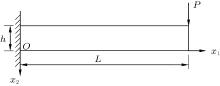
The first example we considered is a cantilever beam subjected to a concentrated load at the free end (see Fig. 1). The length of the beam is L = 8 m, and the height is h = 1 m. The material constants are as follows: the Young’ s modulus E = 105 Pa, the Poisson’ s ratio ν = 0.25, and the yield stress σ s = 25 Pa. The load is P = 1 N.
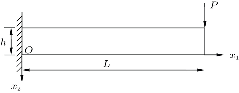 | Fig. 1. Cantilever beam subjected to a concentrated force. |
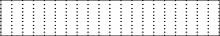
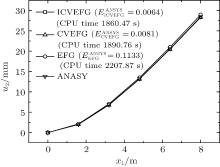
We use the EFG, CVEFG and ICVEFG method to solve this problem. As shown in Fig. 2, 21 × 11 nodes are used. However, in order to obtain better numerical results, 19 × 13 nodes are used in the EFG method. The numerical solutions of the displacement u2 at some nodes and the CPU time using the EFG, CVEFG and ICVEFG method are shown in Fig. 3. By comparing the numerical results obtained using the EFG, CVEFG, and ICVEFG methods, we can see that 


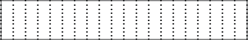 | Fig. 2. Node distribution of the cantilever beam. |
 | Fig. 3. Plots of displacement u2 versus x1 at x2 = L/2. |
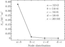
The variation of the displacement with node distribution is shown in Fig. 4. The present results show that the more nodes existing in the domain, the closer to zero the variance is. It means that the ICVEFG method in this paper is convergent.
 | Fig. 4. Variance of the displacement u2 versus node distribution at x2 = 0. |
The relationship between the displacement of midpoint at the end of the beam and the load is shown in Fig. 5. It is obvious that the problem is nonlinear.
 | Fig. 5. Relationship between displacements of midpoint at the end of the beam and the load. |
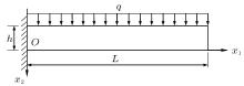
The second example is a cantilever beam subjected to a distributed load (see Fig. 6). The length of the beam is L = 8 m, and the height is h = 1 m. The distributed load is q = 1 N/m. The material constants used in our analysis are Young’ s modulus E = 105 Pa, Poisson’ s ratio ν = 0.25, and the yield stress σ s = 25 Pa.
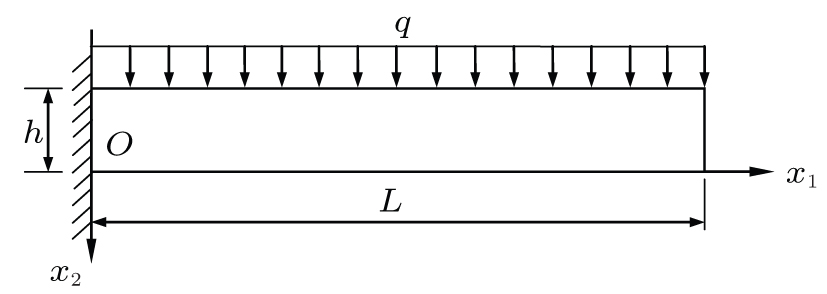 | Fig. 6. Cantilever beam subjected to a distributed load. |
We also use the EFG, CVEFG and ICVEFG method to solve this problem. 21 × 11 nodes are used for the ICVEFG and the CVEFG method in this example as shown in Fig. 2, and 19 × 13 nodes are used in the EFG method. The numerical solutions of the displacement u2 at some nodes are shown in Fig. 7. By comparing with the numerical results obtained using ANSYS, we can also see that the results obtained using the EFG, the CVEFG and the ICVEFG method are in excellent agreement with those obtained using ANSYS. However, the CPU time of the ICVEFG method is less than that of the EFG or the CVEFG method. Then the ICVEFG method in this paper has a greater computational efficiency than the EFG and CVEFG method.
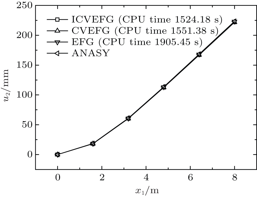 | Fig. 7. Plots of displacement u2 versus x1 at x2 = L/2. |
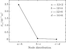
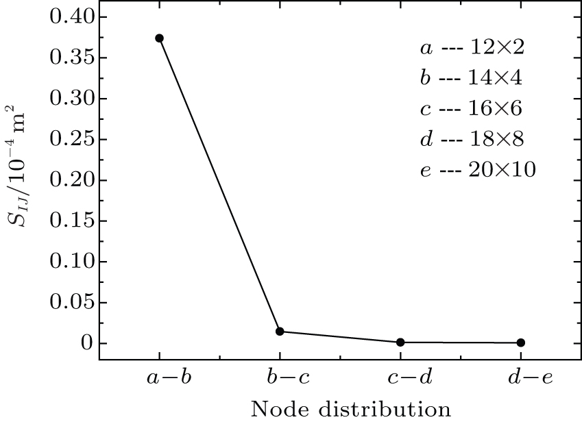
The variances of the displacements under different node distributions are shown in Fig. 8. The present results also show that the more nodes existing in the domain, the closer to zero the variance is. It means that the ICVEFG method in this paper is convergent.
 | Fig. 8. Variance of the displacement u2 versus node distribution at x2 = 0. |
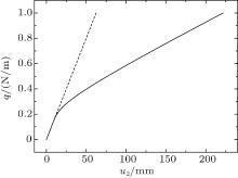
The relationship between the displacements of midpoint at the end of the beam and the load is shown in Fig. 9. It can be seen obviously that the material will enter into the plastic state and the problem is nonlinear.
 | Fig. 9. Relationship between displacements of midpoint at the end of the beam and the load. |
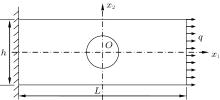
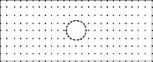
The third example is a rectangular plate with a central hole under a distributed load as shown in Fig. 10. The length of the plate is L = 10 m, the width is h = 4 m, and the radius of the central hole is r = 1 m. The distributed load is q = 1000 N/m. The material constants are as follows: Young’ s modulus E = 1.0 × 10⁵ Pa, Poisson’ s ratio ν = 0.25, and the yield stress σ s = 250 Pa.
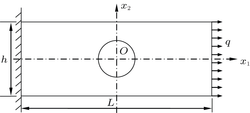 | Fig. 10. A plate with a central hole under a distributed load. |
As shown in Fig. 11, 234 nodes in the domain are used for the ICVEFG and the CVEFG method, and 250 nodes are for the EFG method. The numerical results of the displacement u1 at some nodes, obtained using the EFG, the CVEFG and the ICVEFG method are shown in Table 1. 

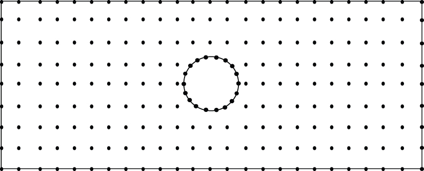 | Fig. 11. Node distribution. |
| Table 1. Elastoplasticity solutions of displacement u1. |
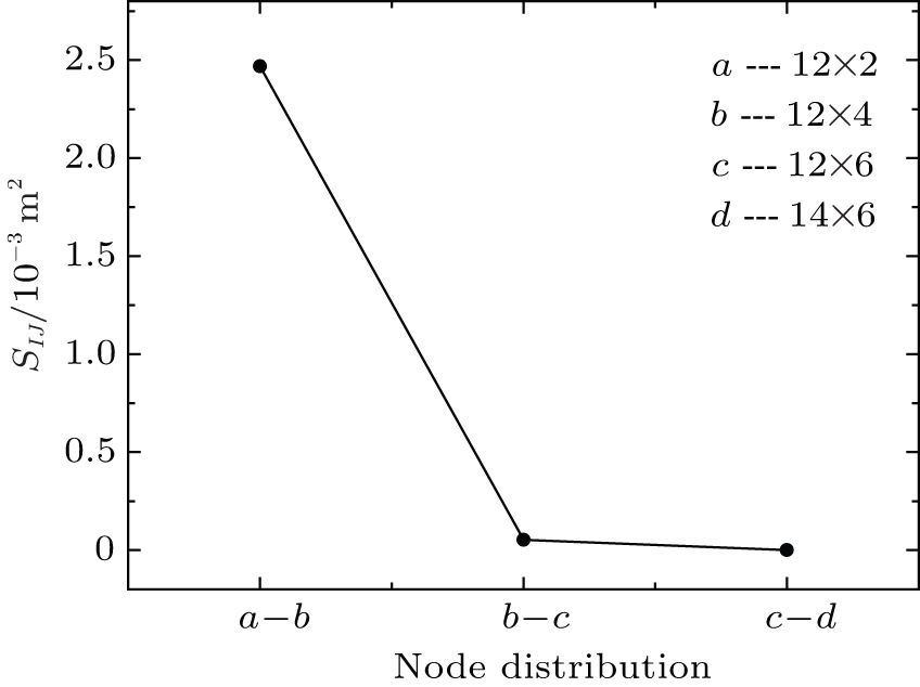
The variances of the displacements under different node distributions are shown in Fig. 12. The present results also show that the more nodes existing in the domain, the closer to zero the variance is. Then it is shown that the ICVEFG method in this paper is convergent.
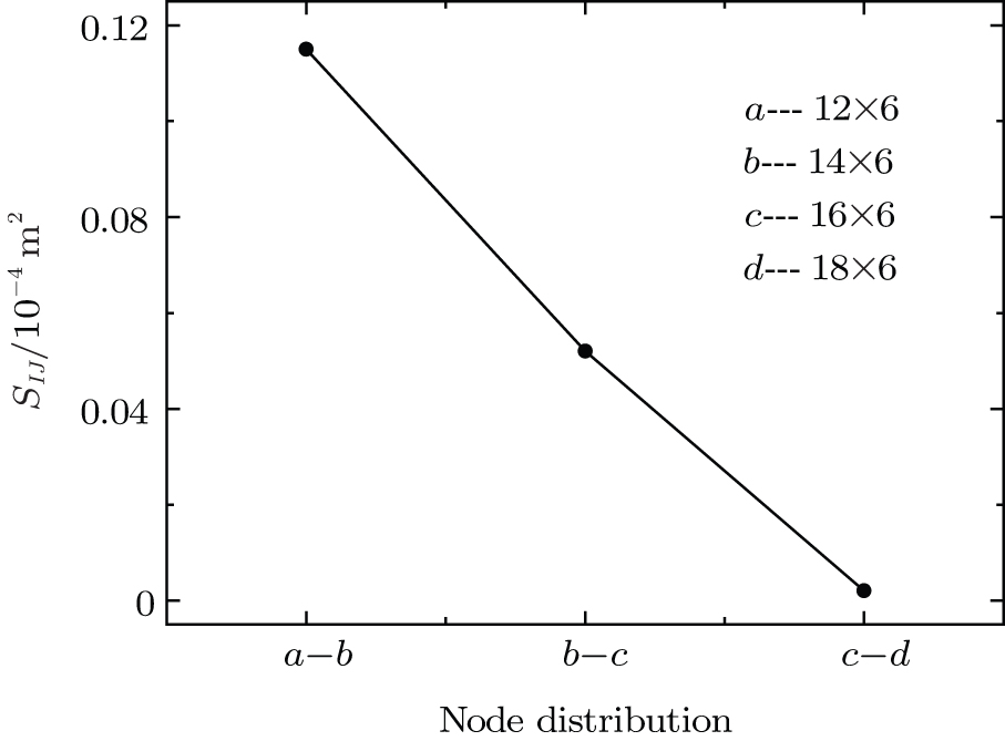 | Fig. 12. Plot of variance of the displacement u2 versus node distribution at x2 = 0. |
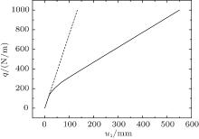
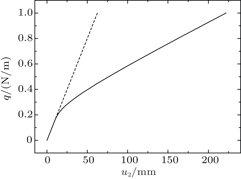
The relationship between the displacements of midpoint at the end of the beam and the load is shown in Fig. 13. Similarly, when the load is larger than the elastic limit, the material begins to yield and enters into the plastic state, which shows the problem is nonlinear.
 | Fig. 13. Relationship between the displacements of midpoint at the right end and the load. |
In this paper, the ICVMLS approximation is used to obtain the shape function, the Galerkin weak form is used to obtain the discretized equation, and the penalty method is used to enforce the displacement boundary conditions, then the ICVEFG method for 2D elastoplasticity problems is presented. Numerical examples are given to show that the ICVEFG method has higher computational precision and efficiency than the EFG and the CVEFG method.
In the ICVMLS approximation, the inverse complex matrix A− 1 is obtained. But the order of the complex matrix is less than that of the matrix in the MLS approximation, and the inverse matrix can be obtained easily.
Because of the limitation of the complex variable theory, the ICVEFG method in this paper can only solve 2D problems. For 3D problems, we can use the meshless methods based on the IMLS approximation.
| 1 |
|
| 2 |
|
| 3 |
|
| 4 |
|
| 5 |
|
| 6 |
|
| 7 |
|
| 8 |
|
| 9 |
|
| 10 |
|
| 11 |
|
| 12 |
|
| 13 |
|
| 14 |
|
| 15 |
|
| 16 |
|
| 17 |
|
| 18 |
|
| 19 |
|
| 20 |
|
| 21 |
|
| 22 |
|
| 23 |
|
| 24 |
|
| 25 |
|
| 26 |
|
| 27 |
|
| 28 |
|
| 29 |
|
| 30 |
|
| 31 |
|
| 32 |
|
| 33 |
|
| 34 |
|
| 35 |
|
| 36 |
|
| 37 |
|
| 38 |
|
| 39 |
|
| 40 |
|
| 41 |
|
| 42 |
|
| 43 |
|
| 44 |
|
| 45 |
|
| 46 |
|
| 47 |
|
| 48 |
|
| 49 |
|
| 50 |
|
| 51 |
|
| 52 |
|
| 53 |
|
| 54 |
|
| 55 |
|
| 56 |
|
| 57 |
|
| 58 |
|
| 59 |
|
| 60 |
|
| 61 |
|
| 62 |
|