Among different centrality measures, each measure has its scope of application and its own characteristic. Here we briefly introduce some classic and authoritative methods, which will be used in experimental analysis in Section  4.

A simple method based on node local properties is degree centrality, namely, the larger degree a node is, the higher influence the node will obtain. Compared with the method based on local properties of nodes, the method considering the global information will give better ranking results, such as betweenness centrality and closeness centrality.

Betweenness is defined as the fraction of shortest paths between node pairs that pass through the nodes of interest. For a network with N nodes, the betweenness centrality of node i, denoted by BC_i is

where g_st is the number of shortest paths between nodes s and t, and denotes the number of shortest paths between s and t which pass through node i.

Closeness of node i is defined as the reciprocal of the average geodesic distances to all other nodes of I, i.e.,

where d_ij is the geodesic distance between i and j.

Another widely employed centrality measure, which can be observed in a natural extension of degree centrality, is eigenvector centrality. Eigenvector centrality^[10] is based on the more subtle notion that a node should be viewed as being influential if it is linked to other nodes which are influential themselves. The eigenvector centrality EC_i of a node i is defined as being proportional to the sum of the eigenvector centralities of the nodes that node i is connected to, i.e.,

where ρ is a constant. It is also assumed that the eigenvector centrality of each node is non-negative (EC_i ≥ 0), for all i.

For a network G with N nodes and M edges, calculating the shortest paths between all pairs of nodes encounters the complexity O(N³) with the Floyd’ s algorithm.^[26] For a sparse graph, it will be more efficient with Johnson’ s algorithm, ^[27] which takes O(N² log_N + NM). For unweighted networks, calculating betweenness centrality encounters O(N²M) using Brandes’ algorithm.^[28]

With the in-depth study on node influence, a growing number of methods^{[17– 21]} have been proposed. Most of these methods are the improved versions of the previous methods and achieve the desired effect. Once the nodes’ influence has already been sorted, the most influential nodes will be used in many fields, such as disease  control  and  prevention in the population, information dissemination in social networks, important power unit protection in the power grid networks, etc. Those applications of influential nodes have gradually improved our lives.

As the era of big data has begun, some novel characteristics have come into being in networks which were ignored in the past, such as extensive, adaptability and time-sensitive. When those characteristics are considered, we have reasons to suspect the availability of the ranking measures. First, rapidly increasing sizes of networks make the information harder to collect, which severely restricts the measures based on the global information. At this point, measures based on local information have greater practical  significance. Second, even just taking local characteristics into consideration, the calculation of all nodes’ centralities is very time-consuming or even not feasible. Meanwhile, the dynamics in networks are very time-sensitive, which means that we need to identify the influential nodes in a very short time. Additionally, many realworld networks are characterized by adaptive changes in their topology depending on the state of their nodes.^[24] The sequence  of  nodes we ranked in the previous time may fail to sort in the present time.

In order to find the influential nodes in less time, we focus our attention on identifying a fraction of high-influence nodes instead of ranking all nodes. Considering the uncertainties of network scale and topology, and the timeliness of dynamic behaviors in real networks, we propose an RIM, which is a method of rapidly identifying high-influence nodes based on the nodes’ local properties. Introduced into this method are the following procedures:

(i) m nodes are randomly chosen as the first source  nodes, denoted as s_i, i = 1, 2, … , m;

(ii) find the highest-degree neighbor of each s_i as the second source nodes, denoted as s_{i_N(1)}, i = 1, 2, … , m, then find the highest-degree neighbor of each s_{i_N(1)} as the third source nodes; according to this method, we will stop when we find the (j + 1) source nodes, denoted as s_{i_N(j)}, i = 1, 2, … , m. In this way, we will find m × j nodes, denoted by s_{i_N(j)}, i = 1, 2, … , m, J = 1, 2, … , j. Note that the first source nodes s_i are not counted, and in the process of finding the highestdegree neighbor of s_{i_N(j)}, if the highest-degree neighbor of s_{i_N(j)} has been found before, we will find the second highestdegree neighbor of s_{i_N(j)};

(iii) rank the m × j nodes according to their degrees, and choose the top-j nodes Tn_j as the target nodes (Tn_j ∈ s_{i_N(j)}).

Considering the fact that the degree is one of the simplest but most important local characteristics of nodes, we can realize our method without knowing the global information about the network. In addition, the close relationship among hubs (high-degree nodes) makes our method effective.

Since the calculating of node i’ s degree requires traversing node i’ s neighborhood within one step, the computational complexity of degree centrality is O(N〈 k〉 ), ^[15] where 〈 k〉 is the average degree of the network. In RIM, we can find m × j target nodes, so the computational complexity of RIM is O(mj〈 k〉 ). Since 〈 k〉 ≪ N, j ≪ N, m ≪ N, we can know that RIM uses much less time than ranking all nodes in the network.

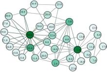
Take Zachary’ s karate club network^[29] for example. There are 34 nodes and 78 edges in the karate network. As shown in Fig.  1, node color becomes deeper as the degree of the node increases. We set m = 1, j = 5, and choose the nodes from the 2nd step to the 6th step as the target nodes. The nodes found by RIM in the karate network and the nodes’ corresponding rankings by degree centrality (DC), betweenness centrality (BC), closeness centrality (CC) and eigenvector centrality (EC) methods for one implementation are shown in Table  1. The computational complexity of degree centrality is O(N〈 k〉 ), and the computational complexity of RIM is O(mj〈 k〉 ). We can see that mj〈 k〉 < N〈 k〉 .

Fig.  1.

	Figure Option ViewDownloadNew Window
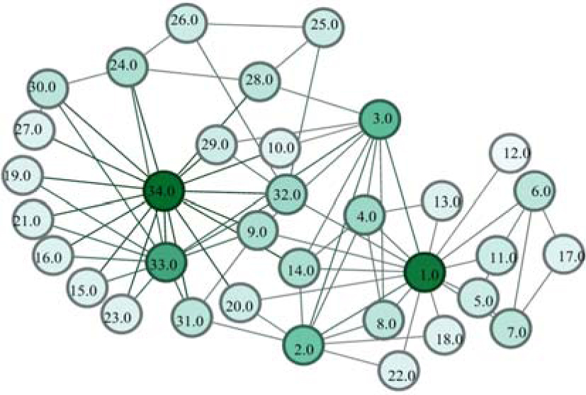	Fig.  1. Zachary’ s karate club network.

Table  1 shows the nodes found by RIM in the karate network in one experiment and the nodes’ corresponding rankings by different centrality methods. According to the  statistics of node rankings, we can see that the target nodes found by RIM have high influence. Almost all top-5 ranking nodes from different methods can be found by RIM in one single experiment. Meanwhile, the appearance number of node n (OT_n) is counted in 500 experiments. In Table  1, it is shown that nodes 1, 3, 33, 34, having high influence verified by different centralities, can almost be found in each of the experiments (OT₁ = 500, OT₃ = 500, OT₃₃ = 489, OT₃₄ = 489).

Table 1.

Table 1.

Table 1. Nodes found by RIM in the karate network and their corresponding rankings obtained from DC, BC, CC and EC methods. Node (n) OTn BC CC DC EC 1 500 1 1 2 5 2 260 7 9 5 5 3 500 4 2 4 3 4 11 15 10 6 8 6 52 10 17 11 25 14 11 8 6 9 7 32 227 5 4 7 9 33 489 3 7 3 4 34 489 2 3 1 1

Table 1. Nodes found by RIM in the karate network and their corresponding rankings obtained from DC, BC, CC and EC methods.

The spreading model is often used for evaluating the performances of the ranking methods.^{[15, 16]} In the following, we use the SIR model to investigate the performances of our method (RIM) in different networks. In the SIR^[25] model, there are three states for a node: i) susceptible (S), ii) infected (I), and iii) recovered (R). S individuals are susceptible to (not yet infected) the disease, I individuals have been infected and are able to spread the disease to susceptible individuals, and R individuals have been recovered and will never be infected any more.

To investigate the influences of target nodes in networks, we set these nodes to be infected initially. The f(t) and F(t) represent the proportion and the number of recovered nodes in the steady state respectively, which can be considered as the indicators to evaluate the influence of the nodes.

In our experiments, we use different artificial networks and real networks to test the effectiveness of our method. The real networks include Facebook, Email and Neural networks. In the Facebook network, we use the Facebook network data of Caltech from a single-time snapshot in September 2005. Only intra-college links are included. There are a total of 769 individuals in this Facebook network, but here we only consider the largest component with 762 individuals. In the email network, the network of e-mail interchanges between members of Rovira i Virgili University (Tarragona)^[30] is used. In the neural network, we use the neural network of C. Elegans, where the data were compiled by Watts and Strogatz.^[31]

The basic topological properties of the networks are shown in Tables  2– 4. In these Tables, N and L are the total numbers of nodes and links, 〈 k〉 denotes the average degree, 〈 d〉 is the average shortest distance, and C and r are the clustering coefficient^[31] and assortative coefficient, ^[32] respectively.

Table 2.

Table 2.

Table 2. Basic topological properties of the real networks. Networks N L 〈 k〉 C 〈 d〉 r Email 1133 5451 9.620 0.0096 3.6060 0.0783 Caltech 762 16651 43.70 0.4093 2.3378 − 0.0662 Neural 297 2148 14.47 0.3080 2.4550 − 0.1632

Table 2. Basic topological properties of the real networks.

Table 3.

Table 3.

Table 3. Basic topological properties of the artificial networks with different structures. Networks N 〈 k〉 C 〈 d〉 r Scale-free network with clustering_1 5000 6 0.009 3.2116 − 0.0052 Scale-free network with clustering_2 5000 6 0.165 3.2573 − 0.0046 Scale-free network with clustering_3 5000 6 0.542 4.5780 − 0.0382 Scale-free network with assortativity_1 5000 6 0.009 3.8629 − 0.050 Scale-free network with assortativity_2 5000 6 0.010 3.8893 0.150 Scale-free network with assortativity_3 5000 6 0.018 4.2205 0.300

Table 3. Basic topological properties of the artificial networks with different structures.

Table 4.

Table 4.

Table 4. Basic topological properties of the artificial networks with different sizes. Networks N 〈 k〉 C 〈 d〉 r Scale-free network_1 1000 6 0.034 3.452 − 0.0813 Scale-free network_2 3000 6 0.014 3.920 − 0.0555 Scale-free network_3 5000 6 0.009 4.079 − 0.0307 Scale-free network_4 7000 6 0.008 4.173 − 0.0395 Scale-free network_5 9000 6 0.006 4.257 − 0.0269

Table 4. Basic topological properties of the artificial networks with different sizes.

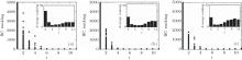
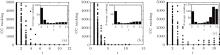
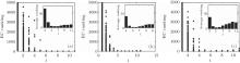
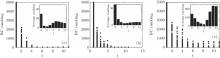
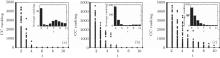
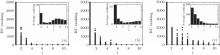
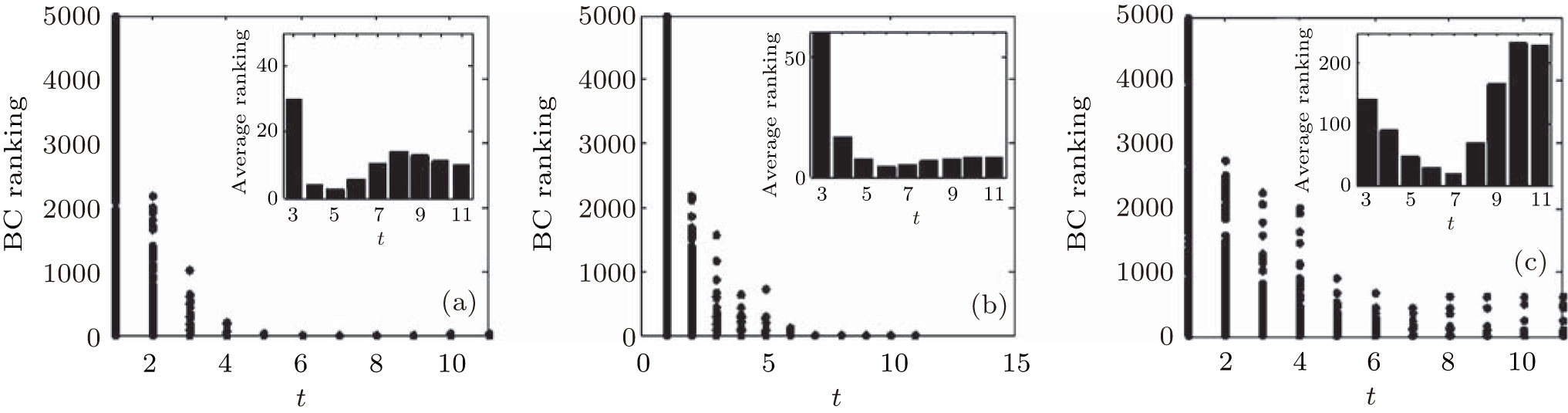
We use different ranking methods to verify the effectiveness of our method. At first, in order to show the results clearly, only one node is randomly selected as the first source node in each implementation, and 10 nodes are found according to our method, which means m = 1, j = 10. After n implementations, the results of node ranking and the average ranking of n implementations in each step t by their corresponding BC, CC, DC, and EC methods in different artificial networks are shown in Figs.  2– 9, including scale-free (SF) networks with different values of the clustering coefficient C (Figs.  2– 5) and the coefficient of assortativity r (Figs.  6– 9).

Fig.  2.

	Figure Option ViewDownloadNew Window
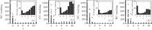
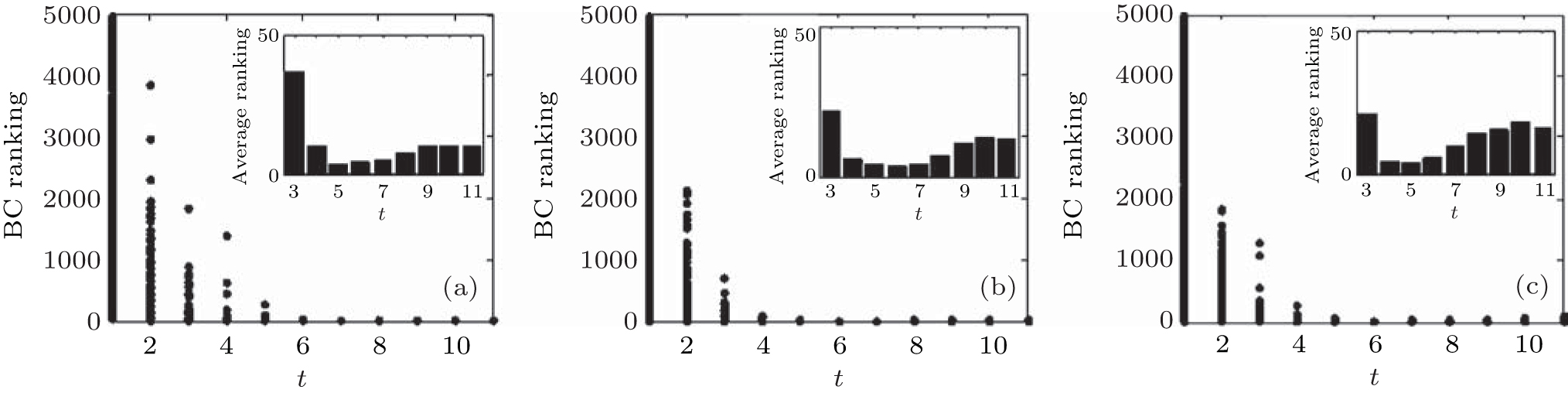	Fig.  2. Target node rankings and the average ranking of 500 implementations by BC for SF networks with the clustering coefficient C = 0.009 (a), 0.165 (b), and 0.542 (c).

Fig.  3.

	Figure Option ViewDownloadNew Window
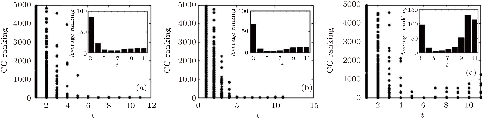	Fig.  3. Target node rankings and the average ranking of 500 implementations by CC for SF networks with the clustering coefficient C = 0.009 (a), 0.165 (b), and 0.542 (c).

Fig.  4.

	Figure Option ViewDownloadNew Window
	Fig.  4. Target node rankings and the average ranking of n = 500 implementations by DC for SF networks with the clustering coefficient C = 0.009 (a), 0.165 (b), and 0.542 (c).

Fig.  5.

	Figure Option ViewDownloadNew Window
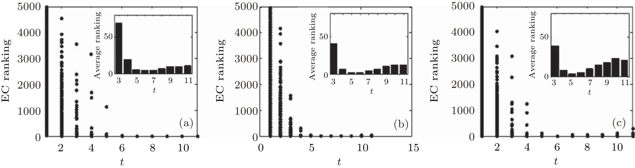	Fig.  5. Target node rankings and the average ranking of 500 implementations by  EC for SF networks with the clustering coefficient C = 0.009 (a), 0.165 (b), and 0.542 (c).

Fig.  6.

	Figure Option ViewDownloadNew Window
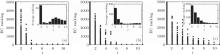
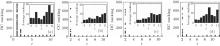
	Fig.  6. Target node rankings and the average ranking of 500 implementations by BC for SF networks with the coefficient of assortativity r = − 0.05 (a), 0.15 (b), and 0.3 (c).

Fig.  7.

	Figure Option ViewDownloadNew Window
	Fig.  7. Target node rankings and the average ranking of 500 implementations by CC for SF networks with the coefficient of assortativity r = − 0.05 (a), 0.15 (b), and 0.3 (c).

Fig.  8.

	Figure Option ViewDownloadNew Window
	Fig.  8. Target node rankings and the average ranking of 500 implementations by DC for SF networks with the coefficient of assortativity r = − 0.05 (a), 0.15 (b), and 0.3 (c).

Fig.  9.

	Figure Option ViewDownloadNew Window
	Fig.  9. Target node rankings and the average ranking of 500 implementations by EC for SF networks with the coefficient of assortativity r = − 0.05 (a), 0.15 (b), and 0.3 (c).

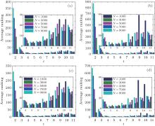
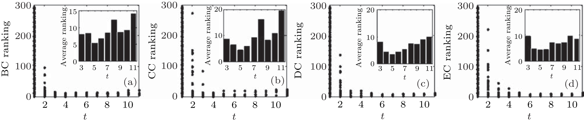
We can see from the figures that the RIM performs well on identifying high-ranking nodes in different networks. Topranking nodes can be identified before the 11th step, and the nodes’ average rankings from the 5th step to the 9th step by different centralities are lower than those in other steps in different network structures, which means that the nodes found from the 5th step to the 9th step are of higher influence. In addition, the experiments in networks with different sizes (Fig.  10) show that the RIM performs well in networks with different sizes.

Fig.  10.

	Figure Option ViewDownloadNew Window
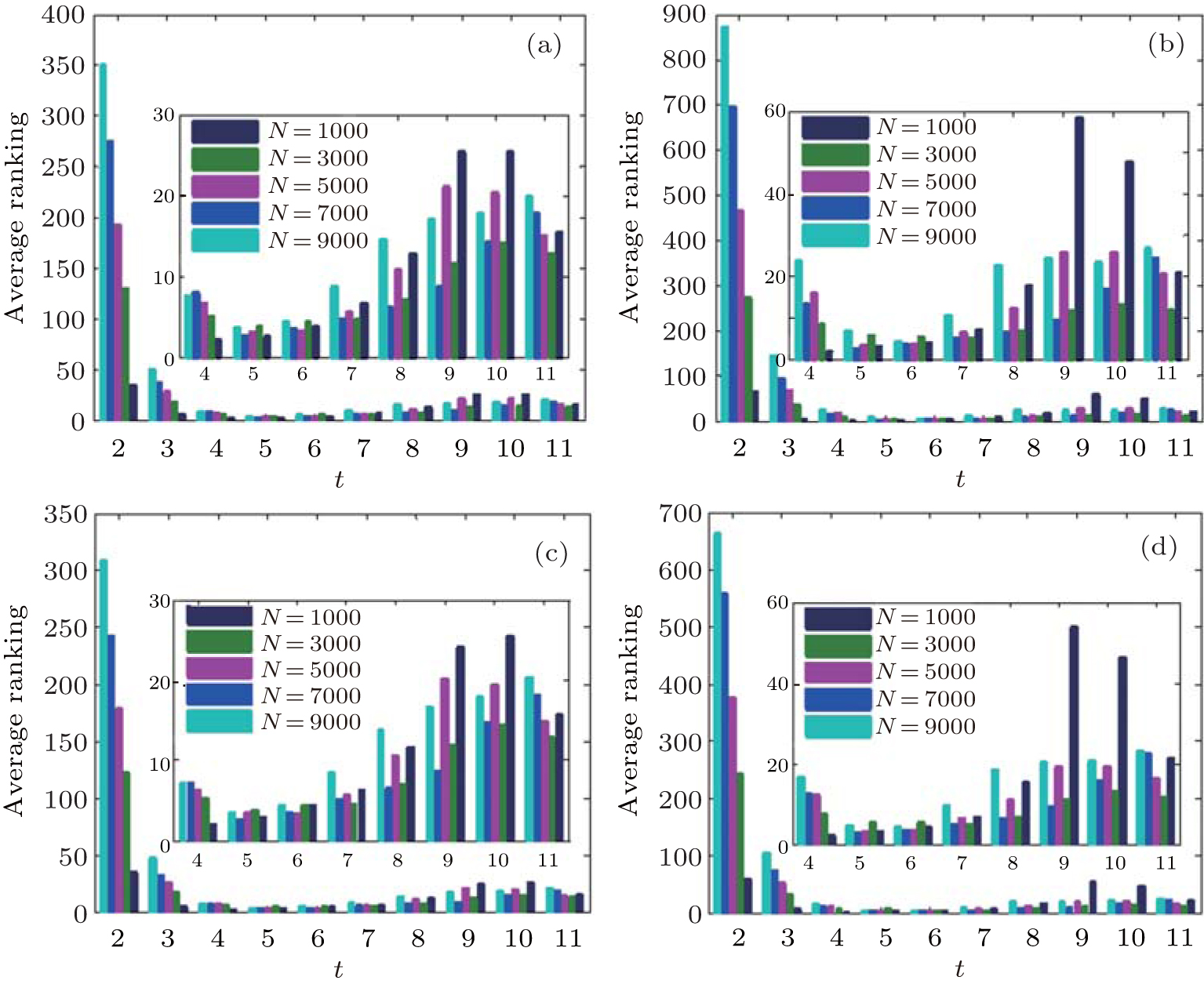	Fig.  10. Target node average ranking of 500 implementations by four different centralities: (a) BC, (b) CC, (c) DC, and (d) EC, for SF networks with different values of scales N.

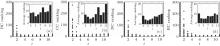
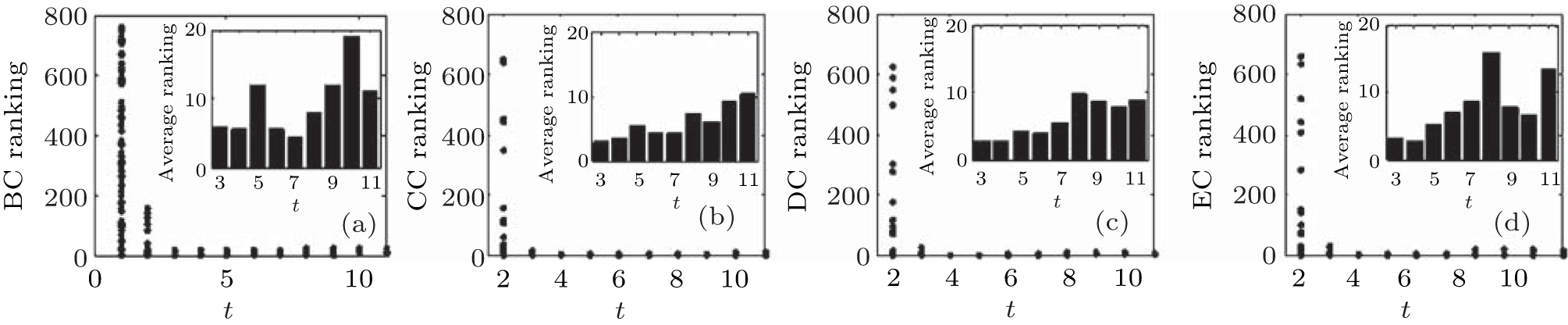
The results in artificial networks show that we can find the highly influential nodes within 10 steps by using the RIM. In each step, only the local information of the node is used, which is more realistic than the ranking measures based on global information. Furthermore, the experiments are also implemented in different real networks, the results of which are shown in Figs.  11– 13. We can see that highly influential nodes can be found within 10 steps, and the nodes’ average rankings from the 4th step to the 8th step by different centralities are lower than those in other steps in different real networks, which means that the nodes found from the 4th step to the 8th step are more influential than other nodes we found.

Fig.  11.

	Figure Option ViewDownloadNew Window
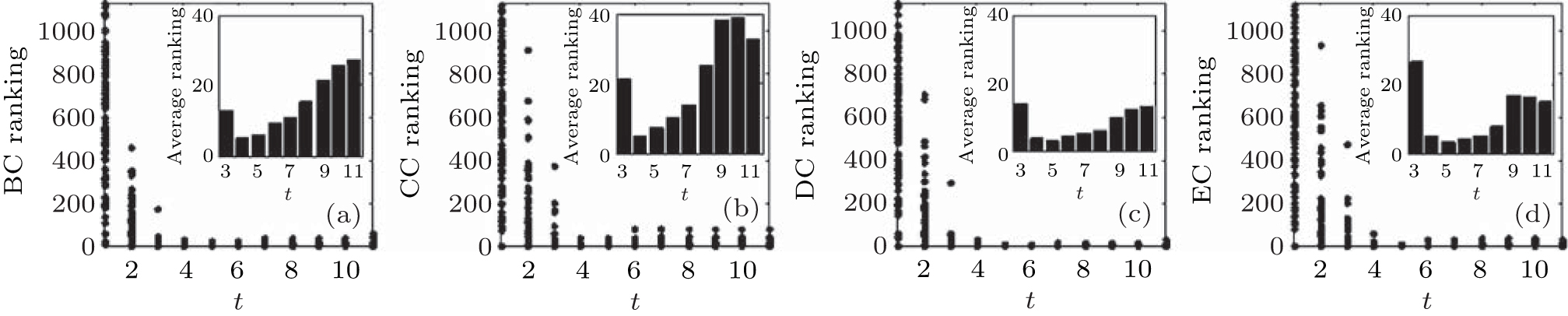	Fig.  11. Target node rankings and the average ranking of 500 implementations for the Email network by four different centralities:, (a) BC, (b) CC, (c) DC, and (d) EC.

Fig.  12.

	Figure Option ViewDownloadNew Window
	Fig.  12. Target node rankings and the average ranking of 500 implementations for the Caltech Facebook network by four different centralities: (a) BC, (b) CC, (c) DC, and (d) EC.

Fig.  13.

	Figure Option ViewDownloadNew Window
	Fig.  13. Target node rankings and the average ranking of 500 implementations for the Neural network by four different centralities: (a) BC, (b) CC, (c) DC, and (d) EC.

We can see from Figs.  2– 13 that under different centrality methods, the influences ranked by different centralities are highly related. For example, the high-influence nodes ranked by degree centrality are relatively high influence under other ranking measures. The top-10 ranked nodes by DC and their corresponding ranks by BC, CC, EC are shown in Table  5. Table  5 shows that top-ranking nodes ranked by different centralities are mostly similar.

Table 5.

Table 5.

Table 5. Top-10 ranked nodes by DC and their corresponding ranks by BC, CC, EC. SF network with assortativity 1 SF network with assortativity 2 SF network with assortativity 3 N DC BC CC EC DC BC CC EC DC BC CC EC 4 1 1 1 1 1 1 1 1 1 1 1 1 2 2 2 2 2 2 2 2 3 2 2 2 3 6 3 3 3 3 3 3 3 2 3 3 3 2 12 4 4 4 4 4 4 4 4 4 4 4 4 9 5 5 5 5 5 5 5 5 5 5 5 5 28 6 8 11 8 6 8 6 6 6 112 8 6 5 7 6 6 6 7 7 13 13 7 629 10 7 8 8 7 7 6 8 6 11 14 8 80 6 10 15 9 11 12 12 9 9 8 8 9 238 11 8 3 10 10 8 7 10 12 10 9 10 516 12 9 SF network with clustering 1 SF network with clustering 2 SF network with clustering 3 N DC BC CC EC N DC BC CC EC N DC BC CC EC 5 1 1 1 1 7 1 4 5 2 4 1 2 2 2 7 2 2 2 2 5 2 5 3 3 5 2 1 1 1 4 3 3 3 3 11 3 2 2 4 8 3 3 4 3 34 4 8 11 8 6 4 1 1 1 6 4 4 5 5 10 5 5 5 5 2 5 6 6 6 3 5 5 3 4 9 6 4 4 4 4 6 3 4 5 39 6 6 7 6 62 7 11 19 15 18 7 7 10 7 16 7 7 9 8 6 8 6 6 6 28 8 8 9 10 9 8 8 15 16 20 9 12 16 12 37 9 10 12 11 12 9 10 11 7 12 10 10 9 9 13 10 9 8 8 7 10 18 10 25 Email network Caltech Facebook network Neural network N DC BC CC EC N DC BC CC EC N DC BC CC EC 105 1 2 3 1 618 1 1 1 1 45 1 1 1 1 333 2 1 1 5 560 2 4 2 2 13 2 2 2 2 16 3 22 40 2 204 3 2 3 6 3 3 3 3 3 23 4 3 2 6 402 4 7 6 5 5 4 5 6 9 42 5 10 4 3 408 5 16 7 4 85 5 12 8 4 41 6 8 5 8 60 6 3 4 14 87 6 8 4 5 196 7 15 19 4 124 7 26 10 3 119 7 15 20 6 233 8 6 7 22 454 8 12 5 7 4 8 7 5 11 21 9 16 20 11 82 9 11 11 11 173 9 10 19 7 76 10 5 6 17 643 10 8 9 13 126 10 11 17 8

Table 5. Top-10 ranked nodes by DC and their corresponding ranks by BC, CC, EC.

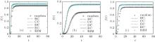
To further evaluate the performance of our method, we use the SIR model to examine the spreading influence of the target nodes. At each step, the susceptible neighbor becomes infected with probability α (here we set α = 0.1). Infected nodes recover with probability β at each step (here we set β = 0.1). To investigate the influence of target nodes found by the RIM, we set these target nodes from the 3rd to the 7th step to be infected initially. By contrast, nodes in the top-5 list by different centrality methods are also treated as infected nodes initially. The ratios of infected nodes to recovered nodes at time t in different artificial networks and real networks, denoted by f (t), are shown in Figs.  14, 15, and 17. In addition, the values of the final number of recovered nodes F(T) in the steady state in networks with different sizes are shown in Fig.  16. Results of Figs.  14– 17 are obtained by averaging over 100 implementations.

Fig.  14.

	Figure Option ViewDownloadNew Window
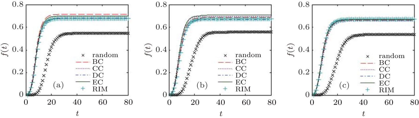	Fig.  14. Infection intensities of nodes as a function of time, with the initially infected nodes found by RIM, compared with the nodes in the top-5 list obtained by different centralities in SF networks with the clustering coefficient C = 0.009 (a), 0.165 (b), and 0.542 (c).

Fig.  15.

	Figure Option ViewDownloadNew Window
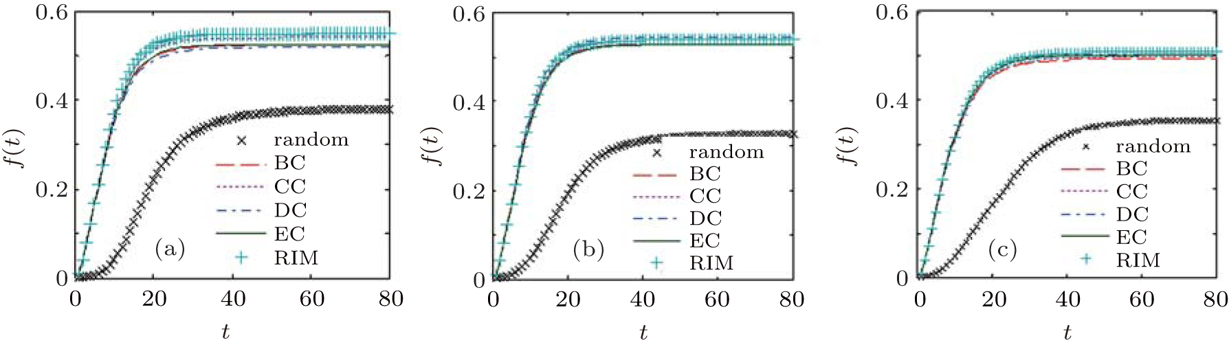	Fig.  15. Infection intensities of nodes as a function of time, with the initially infected nodes found by RIM, compared with the nodes in the top-5 list obtained by different centralities in SF networks with the coefficient of assortativity r = − 0.1 (a), 0 (b), and 0.2 (c).

Fig.  16.

	Figure Option ViewDownloadNew Window
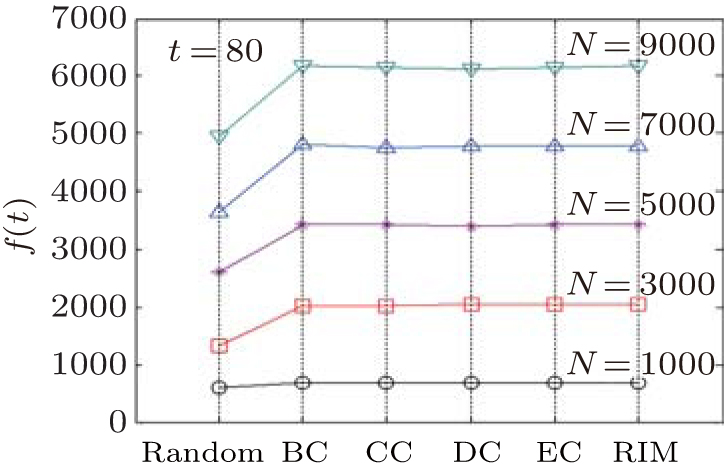	Fig.  16. Infected numbers of the steady state at time t = 80, with the initially infected nodes found by RIM, compared with the nodes in the top-5 list obtained by different centralities in SF networks with different values of size N of networks.

Fig.  17.

	Figure Option ViewDownloadNew Window
	Fig.  17. Infection intensities of nodes as a function of time, with the initially infected nodes found by RIM, compared with the nodes in the top-5 list obtained by different centralities in real networks, i.e., (a) Caltech Facebook network, (b) email network, and (c) neural network.

In Figs.  14– 17, we can see that the curves under different centrality methods are similar to ones under RIM, which means that the nodes found by RIM have almost the same effectiveness on epidemic spreading in different networks, compared with those appearing in the top-5 node list obtained by different centralities. Also we can see that the nodes found by RIM lead to faster and wider spread than in the case that initial spreaders are randomly chosen.